10.4 Time Series Analysis
For time series analysis, there are two data format: ts (time series) and xts (extensible time series). The former needs not have time stamp and can be converted from a vector directly. The latter takes date and time seriously so that it can only be defined with date and/or time columns. We cover the basic time series models, namely, ARMA, GARCH, and VAR.
10.4.1 Time Series data
Function ts convert any vector into time series data.
## Time Series:
## Start = 1
## End = 8
## Frequency = 1
## [1]  2  3  7  8  9 12  8  7
We first define a time series (ts) object for the estimation. Note that ts is similar to xts but without date and time.
## Time Series:
## Start = 1
## End = 3
## Frequency = 1
##   a b d
## 1 3 1 1
## 2 4 2 2
## 3 5 4 3
10.4.2 Extensible Time Series Data
To handle high frequency data (with minute and second), we need the package xts. The package allows you to define Extendible Time Series (xts) object.
The following code installs and loads the xts package.
Consider the following data for our extendible time series
date <- c("2007-01-03","2007-01-04",
          "2007-01-05","2007-01-06",
          "2007-01-07","2007-01-08",
          "2007-01-09","2007-01-10")
time <- c("08:00:01","09:00:01",
          "11:00:01","13:00:01",
          "14:00:01","15:00:01",
          "15:10:01","15:20:03")
price <- c(2,3,7,8,9,12,8,7)
Now we are ready to define xts object. The code as.POSIXct() convert strings into date format with minutes and seconds.
df <-data.frame(date=date, time=time, price=price)
df$datetime <-paste(df$date, df$time)
df$datetime <-as.POSIXct(df$datetime,
                         format="%Y-%m-%d %H:%M:%S")
df <- xts(df,order.by=df$datetime)
For conversion with dates only, we use POSIXlt() instead of POSIXct().
10.4.3 ARMA
Autoregressive moving average model can be estimated using the arima() function.
The following code estimates an AR(1) model:
##
## Call:
## arima(x = price, order = c(1, 0, 0))
##
## Coefficients:
##          ar1  intercept
##       0.6661     6.1682
## s.e.  0.2680     2.1059
##
## sigma^2 estimated as 5.33:  log likelihood = -18.34,  aic = 42.68
The following code estimates an AR(2) model:
##
## Call:
## arima(x = price, order = c(2, 0, 0))
##
## Coefficients:
##          ar1      ar2  intercept
##       0.8301  -0.3026     6.5911
## s.e.  0.3357   0.3638     1.7241
##
## sigma^2 estimated as 4.831:  log likelihood = -18.01,  aic = 44.02
The following code estimates an MA(1) model:
##
## Call:
## arima(x = price, order = c(0, 0, 1))
##
## Coefficients:
##          ma1  intercept
##       0.7945     6.8862
## s.e.  0.4393     1.3412
##
## sigma^2 estimated as 4.936:  log likelihood = -18.23,  aic = 42.46
The following code estimates an MA(2) model:
##
## Call:
## arima(x = price, order = c(0, 0, 2))
##
## Coefficients:
##          ma1     ma2  intercept
##       0.8292  0.1459     6.8262
## s.e.  0.3915  0.3245     1.4677
##
## sigma^2 estimated as 4.945:  log likelihood = -18.14,  aic = 44.28
The following code estimates an ARMA(1,1) model:
##
## Call:
## arima(x = price, order = c(1, 0, 1))
##
## Coefficients:
##          ar1     ma1  intercept
##       0.3551  0.4889     6.6417
## s.e.  0.7701  0.9088     1.8799
##
## sigma^2 estimated as 4.911:  log likelihood = -18.08,  aic = 44.16
Sometimes, we just want to keep the coefficient.
## ar1 ma1 intercept
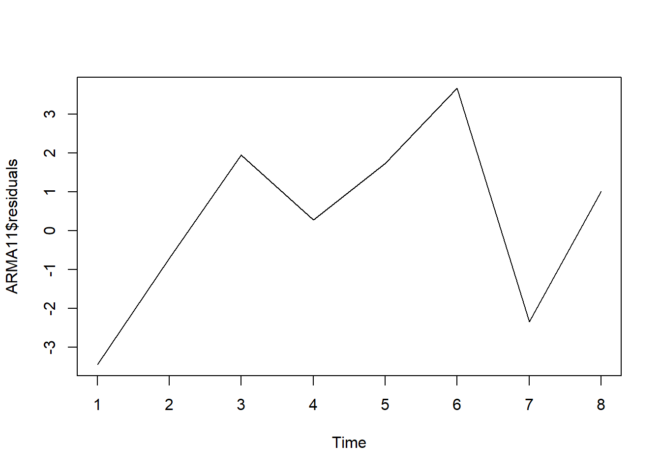
## 0.3551015 0.4889285 6.6417184The following code shows the plot of residuals.
R has a convenient function to autofit() the parameter of ARIMA model. This requires the forecast package. The following code installs and loads the forecast package:
Now we are ready to find the best ARIMA model.
## Series: price
## ARIMA(0,1,0)
##
## sigma^2 estimated as 6.429: log likelihood=-16.45
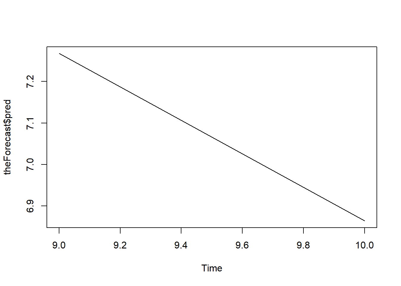
## AIC=34.89 AICc=35.69 BIC=34.84One important function of time series model is forecasting. The following code gives the two-step ahead forecast:
The following shows the forecast plot.
10.4.4 GARCH
To estimate ARCH and GARCH model, we need to install and load package rugarch.
We will estimate GARCH(1,1) with ARMA(1,1) on generate random number
a <- runif(1000, min=0, max=100) #random number

Spec <-ugarchspec(
  variance.model=list(model="sGARCH",
                      garchOrder=c(1,1)),
  mean.model=list(armaOrder=c(1,1)),
  distribution.model="std")
Garch <- ugarchfit(spec=Spec, data=a)
Garch
##
## *---------------------------------*
## * GARCH Model Fit *
## *---------------------------------*
##
## Conditional Variance Dynamics
## -----------------------------------
## GARCH Model : sGARCH(1,1)
## Mean Model : ARFIMA(1,0,1)
## Distribution : std
##
## Optimal Parameters
## ------------------------------------
## Estimate Std. Error t value Pr(>|t|)
## mu 47.87526 0.823773 5.8117e+01 0.000000
## ar1 0.45755 0.308466 1.4833e+00 0.137988
## ma1 -0.51384 0.297101 -1.7295e+00 0.083717
## omega 0.88648 3.099636 2.8599e-01 0.774882
## alpha1 0.00000 0.003760 1.8000e-05 0.999985
## beta1 0.99900 0.000055 1.8287e+04 0.000000
## shape 99.99984 40.329792 2.4796e+00 0.013155
##
## Robust Standard Errors:
## Estimate Std. Error t value Pr(>|t|)
## mu 47.87526 0.841238 5.6910e+01 0.000000
## ar1 0.45755 0.251083 1.8223e+00 0.068405
## ma1 -0.51384 0.240064 -2.1404e+00 0.032320
## omega 0.88648 1.559942 5.6828e-01 0.569847
## alpha1 0.00000 0.001883 3.6000e-05 0.999971
## beta1 0.99900 0.000024 4.1432e+04 0.000000
## shape 99.99984 5.248055 1.9055e+01 0.000000
##
## LogLikelihood : -4782.198
##
## Information Criteria
## ------------------------------------
##
## Akaike 9.5784
## Bayes 9.6127
## Shibata 9.5783
## Hannan-Quinn 9.5915
##
## Weighted Ljung-Box Test on Standardized Residuals
## ------------------------------------
## statistic p-value
## Lag[1] 0.008402 0.9270
## Lag[2*(p+q)+(p+q)-1][5] 0.201723 1.0000
## Lag[4*(p+q)+(p+q)-1][9] 0.922701 0.9999
## d.o.f=2
## H0 : No serial correlation
##
## Weighted Ljung-Box Test on Standardized Squared Residuals
## ------------------------------------
## statistic p-value
## Lag[1] 0.4121 0.5209
## Lag[2*(p+q)+(p+q)-1][5] 2.8914 0.4272
## Lag[4*(p+q)+(p+q)-1][9] 4.8752 0.4480
## d.o.f=2
##
## Weighted ARCH LM Tests
## ------------------------------------
## Statistic Shape Scale P-Value
## ARCH Lag[3] 0.0496 0.500 2.000 0.8238
## ARCH Lag[5] 2.0751 1.440 1.667 0.4549
## ARCH Lag[7] 3.2763 2.315 1.543 0.4630
##
## Nyblom stability test
## ------------------------------------
## Joint Statistic: 210.5276
## Individual Statistics:
## mu 0.4906
## ar1 0.4799
## ma1 0.4632
## omega 0.3867
## alpha1 0.3946
## beta1 0.3800
## shape 34.2276
##
## Asymptotic Critical Values (10% 5% 1%)
## Joint Statistic: 1.69 1.9 2.35
## Individual Statistic: 0.35 0.47 0.75
##
## Sign Bias Test
## ------------------------------------
## t-value prob sig
## Sign Bias 0.2600 0.7949
## Negative Sign Bias 0.8307 0.4064
## Positive Sign Bias 0.2381 0.8119
## Joint Effect 1.4191 0.7011
##
##
## Adjusted Pearson Goodness-of-Fit Test:
## ------------------------------------
## group statistic p-value(g-1)
## 1 20 240.2 3.023e-40
## 2 30 241.2 2.517e-35
## 3 40 251.3 7.715e-33
## 4 50 308.0 3.136e-39
##
##
## Elapsed time : 0.2583098To obtain specific result of the GARCH model, we use the following code:
10.4.5 VAR
The following data will be used to estimate VAR model.
a<- c(3.1,3.4,5.6,7.5,5,6,6,7.5,4.5,
      6.7,9,10,8.9,7.2,7.5,6.8,9.1)
b <- c(3.2,3.3,4.6,8.5,6,6.2,5.9,7.3,
       4,7.2,3,12,9,6.5,5,6,7.5)
d <-c(4,6.2,5.3,3.6,7.5,6,6.2,6.9,
      8.2,4,4.2,5,11,3,2.5,3,6)
df <-data.frame(a,b,d)
To estimate a VAR model, we need to install and load vars packages.
The following code estimates the VAR(2) model.
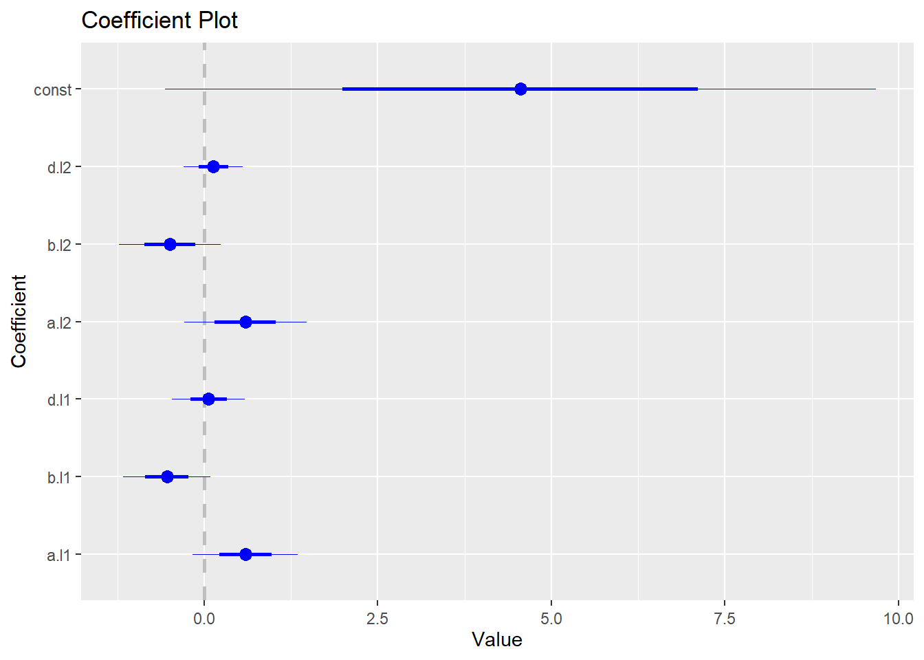
## $a
## Estimate Std. Error t value Pr(>|t|)
## a.l1 0.59366615 0.3776796 1.5718776 0.1546224
## b.l1 -0.53728016 0.3153665 -1.7036692 0.1268463
## d.l1 0.06427631 0.2620526 0.2452802 0.8124144
## a.l2 0.59478214 0.4406631 1.3497434 0.2140455
## b.l2 -0.49271501 0.3681374 -1.3383999 0.2175550
## d.l2 0.13247171 0.2139979 0.6190328 0.5531098
## const 4.55502873 2.5585550 1.7803130 0.1128965
##
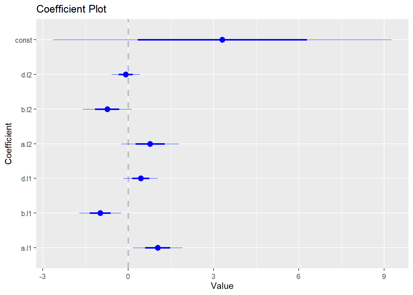
## $b
## Estimate Std. Error t value Pr(>|t|)
## a.l1 1.03577283 0.4390665 2.3590341 0.04602757
## b.l1 -0.98047999 0.3666252 -2.6743391 0.02817211
## d.l1 0.43849071 0.3046458 1.4393458 0.18800763
## a.l2 0.77048414 0.5122871 1.5040084 0.17098968
## b.l2 -0.74120465 0.4279733 -1.7318948 0.12153171
## d.l2 -0.08577585 0.2487804 -0.3447853 0.73914487
## const 3.30736245 2.9744145 1.1119373 0.29846082
##
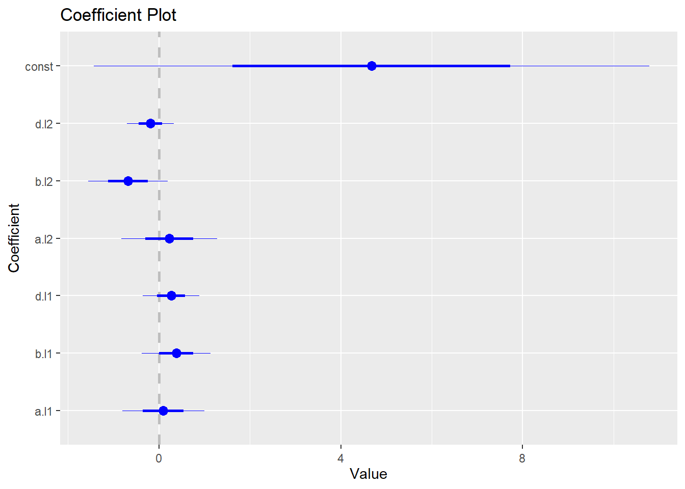
## $d
## Estimate Std. Error t value Pr(>|t|)
## a.l1 0.09567126 0.4508959 0.2121804 0.8372726
## b.l1 0.37908977 0.3765028 1.0068710 0.3434765
## d.l1 0.26703079 0.3128536 0.8535327 0.4181858
## a.l2 0.23097179 0.5260892 0.4390354 0.6722522
## b.l2 -0.67987321 0.4395038 -1.5469110 0.1604714
## d.l2 -0.18657598 0.2554831 -0.7302869 0.4860477
## const 4.67527066 3.0545515 1.5305915 0.1644018##
## VAR Estimation Results:
## =========================
## Endogenous variables: a, b, d
## Deterministic variables: const
## Sample size: 15
## Log Likelihood: -71.865
## Roots of the characteristic polynomial:
## 0.8034 0.8034 0.6583 0.6583 0.4639 0.4639
## Call:
## VAR(y = df, p = 2)
##
##
## Estimation results for equation a:
## ==================================
## a = a.l1 + b.l1 + d.l1 + a.l2 + b.l2 + d.l2 + const
##
## Estimate Std. Error t value Pr(>|t|)
## a.l1 0.59367 0.37768 1.572 0.155
## b.l1 -0.53728 0.31537 -1.704 0.127
## d.l1 0.06428 0.26205 0.245 0.812
## a.l2 0.59478 0.44066 1.350 0.214
## b.l2 -0.49272 0.36814 -1.338 0.218
## d.l2 0.13247 0.21400 0.619 0.553
## const 4.55503 2.55856 1.780 0.113
##
##
## Residual standard error: 1.552 on 8 degrees of freedom
## Multiple R-Squared: 0.4615, Adjusted R-squared: 0.0576
## F-statistic: 1.143 on 6 and 8 DF, p-value: 0.4184
##
##
## Estimation results for equation b:
## ==================================
## b = a.l1 + b.l1 + d.l1 + a.l2 + b.l2 + d.l2 + const
##
## Estimate Std. Error t value Pr(>|t|)
## a.l1 1.03577 0.43907 2.359 0.0460 *
## b.l1 -0.98048 0.36663 -2.674 0.0282 *
## d.l1 0.43849 0.30465 1.439 0.1880
## a.l2 0.77048 0.51229 1.504 0.1710
## b.l2 -0.74120 0.42797 -1.732 0.1215
## d.l2 -0.08578 0.24878 -0.345 0.7391
## const 3.30736 2.97441 1.112 0.2985
## ---
## Signif. codes: 0 '***' 0.001 '**' 0.01 '*' 0.05 '.' 0.1 ' ' 1
##
##
## Residual standard error: 1.805 on 8 degrees of freedom
## Multiple R-Squared: 0.616, Adjusted R-squared: 0.328
## F-statistic: 2.139 on 6 and 8 DF, p-value: 0.1578
##
##
## Estimation results for equation d:
## ==================================
## d = a.l1 + b.l1 + d.l1 + a.l2 + b.l2 + d.l2 + const
##
## Estimate Std. Error t value Pr(>|t|)
## a.l1 0.09567 0.45090 0.212 0.837
## b.l1 0.37909 0.37650 1.007 0.343
## d.l1 0.26703 0.31285 0.854 0.418
## a.l2 0.23097 0.52609 0.439 0.672
## b.l2 -0.67987 0.43950 -1.547 0.160
## d.l2 -0.18658 0.25548 -0.730 0.486
## const 4.67527 3.05455 1.531 0.164
##
##
## Residual standard error: 1.853 on 8 degrees of freedom
## Multiple R-Squared: 0.6278, Adjusted R-squared: 0.3487
## F-statistic: 2.249 on 6 and 8 DF, p-value: 0.143
##
##
##
## Covariance matrix of residuals:
## a b d
## a 2.4097 0.7713 -1.0454
## b 0.7713 3.2566 0.6701
## d -1.0454 0.6701 3.4345
##
## Correlation matrix of residuals:
## a b d
## a 1.0000 0.2753 -0.3634
## b 0.2753 1.0000 0.2004
## d -0.3634 0.2004 1.0000To generate coefficient plot, we need to install and load coefplot package:
The following code generates the coefficient plot for the VAR model: