5.4 Bollinger band

A channel (or band) is an area that surrounds a trend within which price movement does not indicate formation of a new trend.

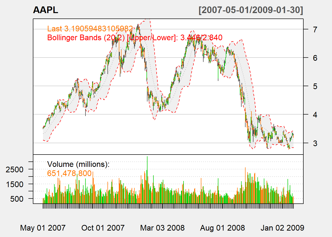
For Bollinger band, channel is drawn over a trend line plus/minus 2 standard deviation (SD).

Trend line: SMA or EMA of price (price can be closing price or average of high, low, and close)

Bandwidth: determined by the asset volatility \[B_t(n)=k\times stdev(P_t, n)\] where usually we have \(k=2\) and \(n=20\).

The lower and upper bands are \[up_t = P_t + B_t(n) \text{, and } down_t=P_t - B_t(n).\]

To denote the location of the price, we use \[\%B=\frac{P_t-down_t}{up_t-down_t}\]

where it is greater 1 if it is above the upper band, and less than 0 when it is below the lower band.

myBBands <- function (price,n,sd){
  mavg <- SMA(price,n)
  sdev <- rep(0,n)
  N <- nrow(price)
  for (i in (n+1):N){
    sdev[i]<- sd(price[(i-n+1):i])
  }
  up <- mavg + sd*sdev
  dn <- mavg - sd*sdev
  pctB <- (price - dn)/(up - dn)
  output <- cbind(dn, mavg, up, pctB)
  colnames(output) <- c("dn", "mavg", "up", 
        "pctB")
  return(output)
}

Now let us put our code to work:

bb <-myBBands(Cl(AAPL),n=20,sd=2)
tail(bb,n=5)

##                  dn     mavg       up      pctB
## 2012-12-21 17.59272 19.61250 21.63228 0.2363574
## 2012-12-24 17.53862 19.48864 21.43866 0.2663760
## 2012-12-26 17.46053 19.36046 21.26040 0.2265595
## 2012-12-27 17.42374 19.23925 21.05476 0.2674896
## 2012-12-28 17.43880 19.09680 20.75481 0.2294458

5.4.1 TTR

We use BBands in TTR to calculate:

bb <-BBands(Cl(AAPL),n=20, sd=2)
tail(bb,n=5)

##                  dn     mavg       up      pctB
## 2012-12-21 17.64386 19.61250 21.58114 0.2295084
## 2012-12-24 17.58800 19.48864 21.38929 0.2603068
## 2012-12-26 17.50864 19.36046 21.21229 0.2194560
## 2012-12-27 17.46971 19.23925 21.00879 0.2614493
## 2012-12-28 17.48078 19.09680 20.71283 0.2224172

Note that it is different from above. It turns out that the standard deviation used is population instead of sample one. We only need to correct it by the factor of \(\sqrt{(n-1)/n}\).

myBBands <- function (price,n,sd){
  mavg <- SMA(price,n)
  sdev <- rep(0,n)
  N <- nrow(price)
  for (i in (n+1):N){
    sdev[i]<- sd(price[(i-n+1):i])
  }
  sdev <- sqrt((n-1)/n)*sdev
  up <- mavg + sd*sdev
  dn <- mavg - sd*sdev
  pctB <- (price - dn)/(up - dn)
  output <- cbind(dn, mavg, up, pctB)
  colnames(output) <- c("dn", "mavg", "up", 
        "pctB")
  return(output)
}

Now we can reoncile the two:

bb <-myBBands(Cl(AAPL),n=20,sd=2)
tail(bb,n=5)

##                  dn     mavg       up      pctB
## 2012-12-21 17.64386 19.61250 21.58114 0.2295084
## 2012-12-24 17.58800 19.48864 21.38929 0.2603068
## 2012-12-26 17.50864 19.36046 21.21229 0.2194560
## 2012-12-27 17.46971 19.23925 21.00879 0.2614493
## 2012-12-28 17.48078 19.09680 20.71283 0.2224172

5.4.2 Trading Signal

Buy signal arises when price is above the band.

Sell signal arises when price is below the band.

5.4.3 Charting

chartSeries(AAPL,
            subset='2007-05::2009-01',
            theme=chartTheme('white'))
addBBands(n=20,sd=2)