7.2 Simple filter buy rule
Here we create trading signal based on simple filter rule. Recall that simple filter rule suggests buying when the price increases a lot compared to the yesterday price: \[\begin{align*} \text{Buy}&:\frac{P_t}{P_{t-1}}>1+\delta \\ \end{align*}\] where \(P_t\) is the closing price at time \(t\) and \(\delta>0\) is an arbitrary threshold
We illustrate using Microsoft with ticker MSFT.
We first download the data using getSymbols(“MSFT”).
## [1] "MSFT"We first will use closing price to perform calculation. We calculate the percentage price change by dividing the current close price by its own lag and then minus 1.
Now we generate buying signal based on filter rule:
price <- Cl(MSFT) # close price
r <- price/Lag(price) - 1 # % price change
delta <-0.005 #threshold
signal <-c(0) # first date has no signal

#Loop over all trading days (except the first)
for (i in 2: length(price)){
  if (r[i] > delta){
    signal[i]<- 1
  } else
    signal[i]<- 0
}
Note that signal is just a vector without time stamp. We use the function reclass to convert it into an xts object.
## [1] 0 0 0# Assign time to action variable using reclass
signal<-reclass(signal,price)
# Each point is now attached with time
tail(signal, n=3)## [,1]
## 2021-05-05 0
## 2021-05-06 1
## 2021-05-07 1We are now ready to chart the trading indicators:
# Charting with Trading rule
chartSeries(MSFT,
            type = 'line',
            subset="2009-08::2009-09-15",
            theme=chartTheme('white'))
addTA(signal,type='S',col='red')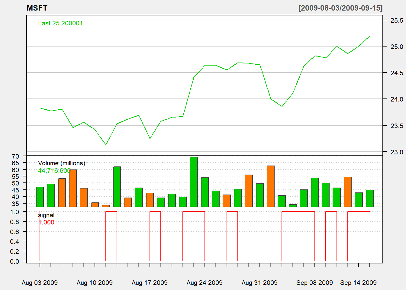
We consider trading based on yesterday indicator:
We may evaluate this trading signal using day trading:
- buy at open
- sell at close
- trading size: all in
Then daily net return percentage is \(\frac{Close - Open}{open}\).
Note that sometimes we can make approximate returnMSFT using \(dailyReturn_t=\frac{Close_{t} - Close_{t-1}}{Close_{t-1}}\) because daily return is available using dailyReturn() in quantmod.
Based on daily return of the portfolio, we will draw three basic charts:
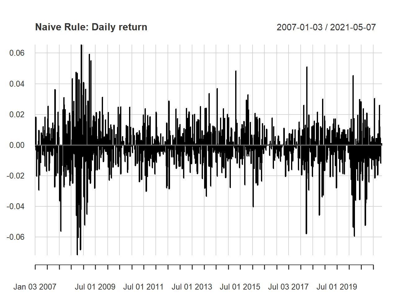
- a chart of daily return
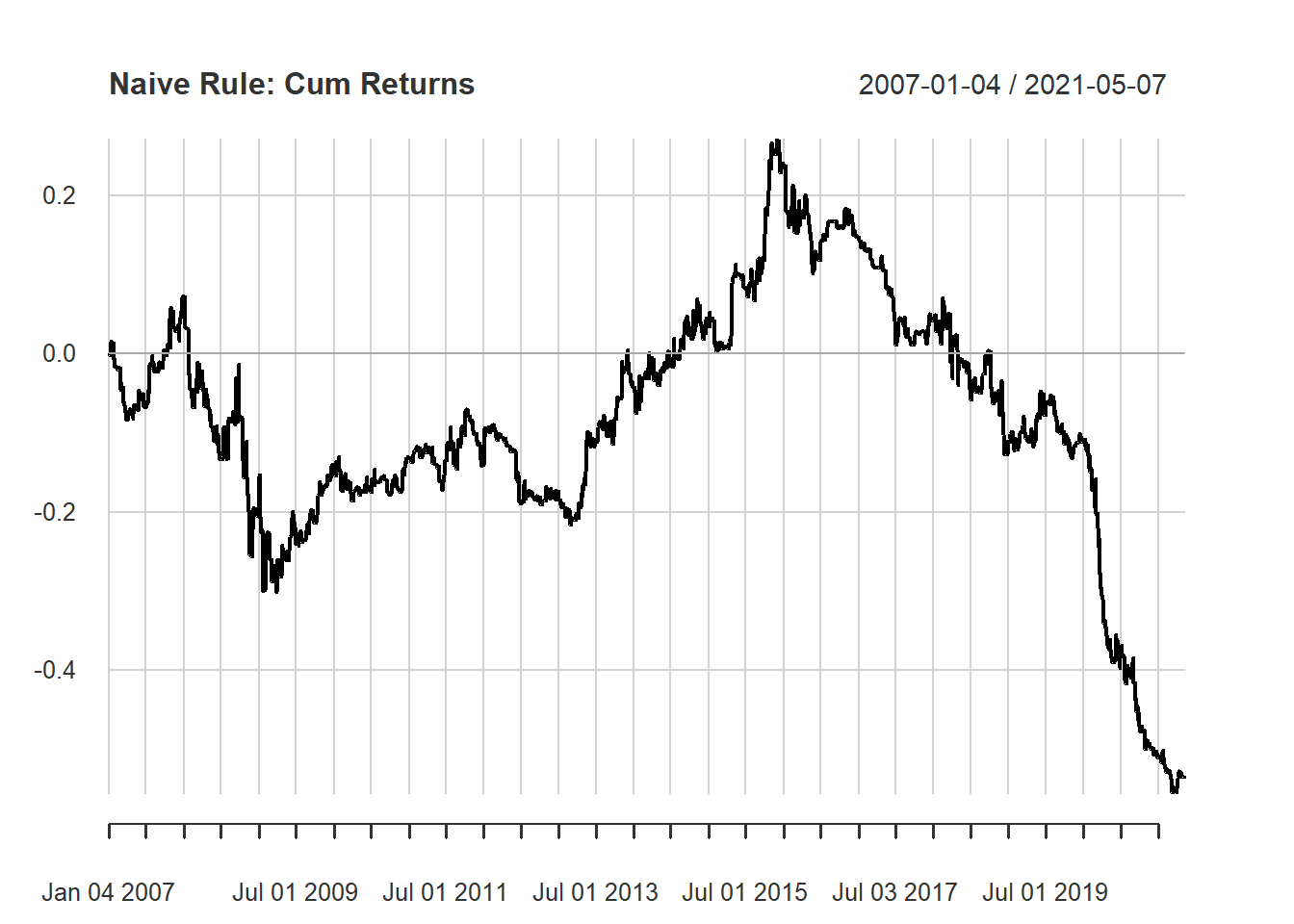
- a chart of cumulative return
- a chart of drawdown
The function chart.Bar is a line chart of return. Since our data is in daily frequency, we will have a chart of daily return.
The function chart.CumReturns is a line chart of cumulative (net) return. The default option is in geometric style: \[Cum.Return_{t}=wealth.index_t-1\] where \(R_t\) is return of day \(t\) and \(wealth.index_t =(1+R_1)\times...\times(1+R_t)\). When it is positive, there is a profit. Simialrly, when it is negative, there is a loss.
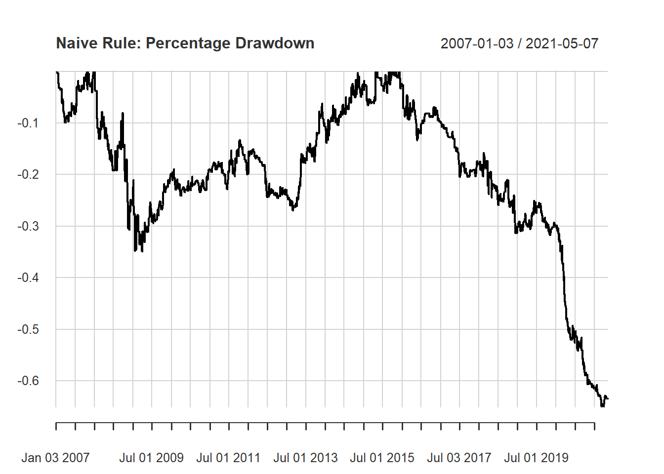
The function chart.Drawdown is a line chart of percentage drawndown. Histroical drawdown is the current distance from the historical maximum value. It is a measure of how risky of the investment strategy. In formula, we have \[Drawdown_t=wealth.index_t-hist.high_t\] where \(hist.high_t=max\{wealth.index_1,...,wealth.index_t\}\) Hence, percentage drawdown is \[Percentage.Drawdown_t=\frac{wealth.index_t}{hist.high_t}-1\]
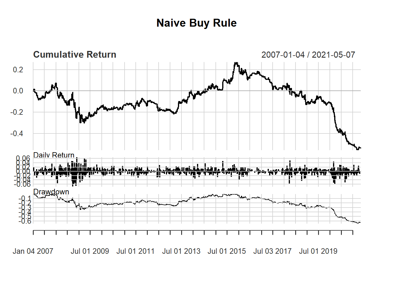
Finally, we can see the summary of performance using charts.PerformanceSummary() to evaluate the performance.