22 Tutorial 7: The Central Limit Theorem
The central limit theorem states that when samples of larger and larger sizes are drawn with replacement from a population, the distribution of the sample means (the sampling distribution) of equally sized samples will become increasingly normal as the sample size increases. This tendency tends to become apparent for a sample size of n >= 30. This is true regardless of the distribution of the underlying variable.
I will offer a few examples below to demonstrate this, focusing on distributions that do not resemble the normal distribution in order to make this theorem more clear.
First we’ll look at an example using the exponential distribution. We’ll do this using a function called clt_plot_exp() which takes two arguments. The first, n, is the size of the samples in the sampling distribution we want to plot. The second, trials, is the number of samples we want to draw. The function produces a grid of four plots which show the probability density function (PDF) for this variable, the distribution of a single large sample of this variable (sample distribution), a histogram of samples of size n of this distribution (sampling distribution) and a qq plot of the sampling distribution. The top row of the grid focuses on individual observations and the bottom row focuses on samples. We’re going to run this function for n = 100 and trials = 1000.
clt_plot_exp <- function(n, trials){
  pdf <- function(x){
    ifelse(x == 0, 0, (1 / 10) * exp(-x / 10))
  }
  dat <- data.frame(x = seq(0.01, 25, 2.25),
                    prob = pdf(seq(0.01, 25, 2.25)))
  mean_data <- as.numeric(replicate(trials, mean(sample(dat$x,
                                                        n,
                                                        replace = TRUE,
                                                        prob = dat$prob))))
  mean_frame <- data.frame(x = length(0:(length(mean_data) - 1)),
                           samp = mean_data)
  sampling_dist <- as.data.frame(scale(mean_frame)) %>% ggplot(aes(samp, stat(count / sum(count)))) +
    geom_histogram(color = 'black',
                   fill = 'blue',
                   bins = 10) +
    labs(x = 'Number of standard deviations',
         y = 'Proportion',
         title = 'Sampling distribution') +
    geom_vline(xintercept = 0, color = 'red',
               linetype = 'dashed', size = 1) + ds_theme_set()
  qq <- as.data.frame(scale(mean_frame)) %>% ggplot(aes(sample = samp)) +
    stat_qq(color = 'blue', alpha = 0.5) +
    stat_qq_line() +
    labs(title = 'QQ plot') + ds_theme_set()
  pdf <- dat %>% ggplot(aes(x)) +
    stat_function(fun = pdf, size = 1) +
    scale_y_continuous(limits = c(0, max(dat$prob) + 0.05)) +
    labs(title = 'PDF') + ds_theme_set()
  samp_dist <- dat %>% ggplot(aes(x, prob)) +
    geom_bar(stat = 'identity',
             color = 'black',
             fill = 'red') +
    labs(y = 'Probability',
         x = 'x',
         title = 'Sample distribution') + ds_theme_set()
  ggarrange(pdf, samp_dist, sampling_dist, qq, ncol = 2, nrow = 2)
}

clt_plot_exp(100, 1000)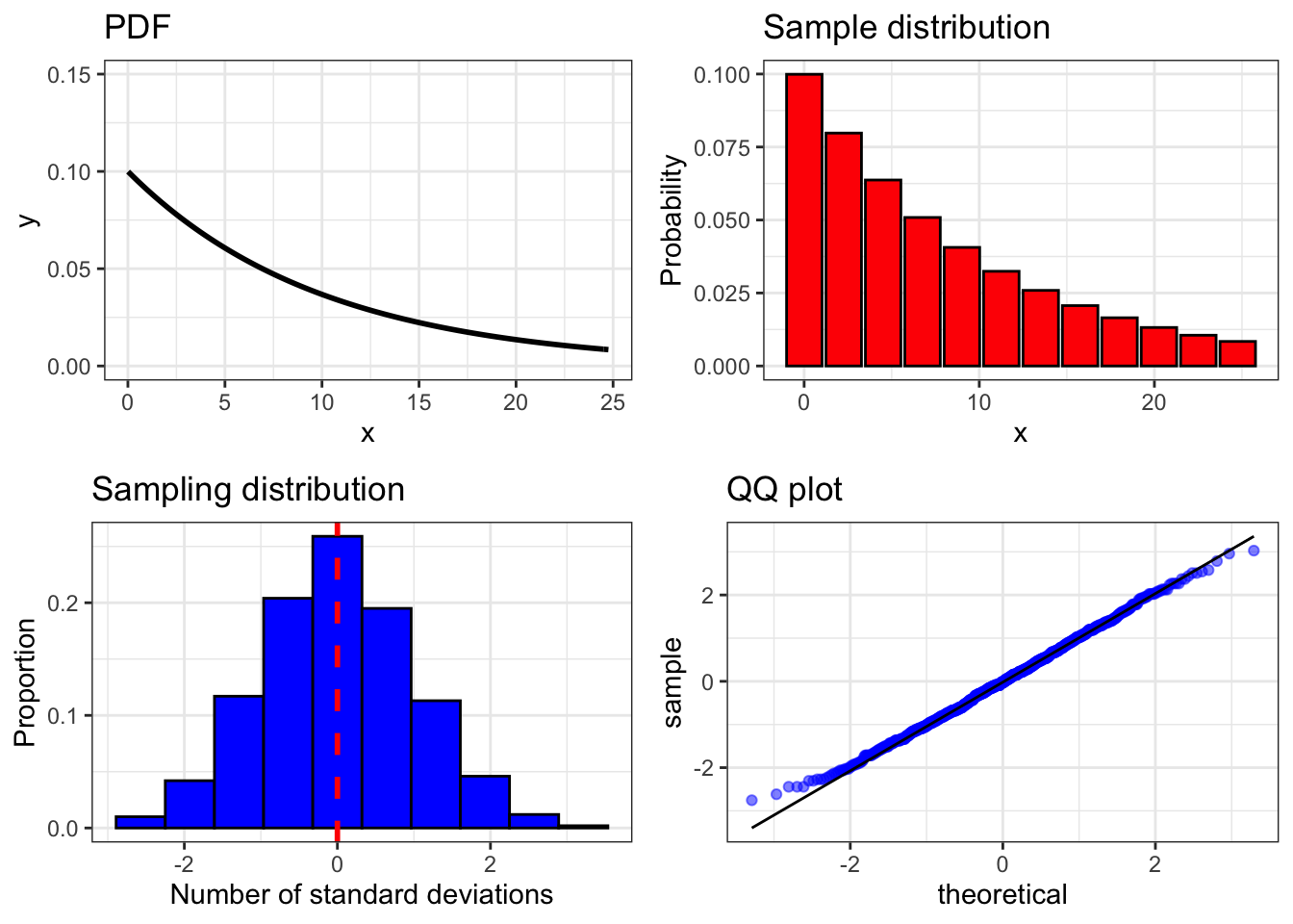
Notice how different the shapes of the plots which relate to individual observations are from the ones that relate to samples which are drawn from the same distribution. It bears repeating that according to the central limit theorem, it does not matter how individual observations of a random variable are distributed because when samples of larger and larger sizes are drawn with replacement from this population, the distribution of the means of a large number of equally sized samples will look increasingly normal. That is reflected above in the sampling distribution and the qq plot of sample means.
Now let’s try this one more time. This time we’ll use the uniform distribution. We’ll do this using a function called clt_plot_unif() which takes two arguments, n and trials, that mean the same thing as in the last function we used.
clt_plot_unif <- function(n, trials){
  dat <- data.frame(x = seq(0, 10, 1),
                    prob = dunif(n, 0, 10))
  mean_data <- as.numeric(replicate(trials, mean(sample(dat$x, n, replace = TRUE, prob = dat$prob))))
  mean_frame <- data.frame(x = length(0:(length(mean_data) - 1)),
                           samp = mean_data)
  sampling_dist <- as.data.frame(scale(mean_frame)) %>% ggplot(aes(samp, stat(count / sum(count)))) +
    geom_histogram(color = 'black',
                   fill = 'blue',
                   bins = 10) +
    labs(x = 'Number of standard deviations',
         y = 'Proportion',
         title = 'Sampling distribution') +
    geom_vline(xintercept = 0,
               color = 'red',
               linetype = 'dashed',
               size = 1) + ds_theme_set()
  qq <- as.data.frame(scale(mean_frame)) %>% ggplot(aes(sample = samp)) +
    stat_qq(color = 'blue',
            alpha = 0.5) +
    stat_qq_line() +
    labs(title = 'QQ plot') + ds_theme_set()
  pdf <- dat %>% ggplot(aes(x, prob)) +
    geom_line(size = 1) +
    scale_y_continuous(limits = c(0, max(dat$prob) + 0.05)) +
    labs(title = 'PDF') + ds_theme_set()
  samp_dist <- dat %>% ggplot(aes(x, prob)) +
    geom_bar(stat = 'identity',
             color = 'black',
             fill = 'red') +
    labs(y = 'Probability', x = 'x',
         title = 'Sample distribution') + ds_theme_set()
  ggarrange(pdf, samp_dist, sampling_dist, qq, ncol = 2, nrow = 2)
}

clt_plot_unif(10, 1000)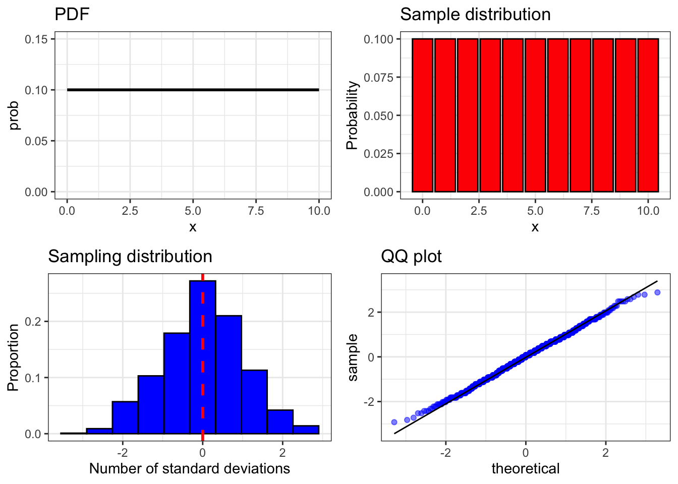
Once again, because of the central limit theorem, we see that a random variable whose individual observations clearly do not follow a normal distribution still has a normally distributed sampling distribution. We could repeat this for many other distributions, such as chi squared, the binomial distribution, the Poisson distribution and so on. The results would be the same.
22.0.1 Simulating jury pools from Swain v. Alabama
This simulation is adapted from a lecture given by Ani Adhikari in the online, low-cost/free version of Data Science 8, a course offered at the University of California, Berkeley. In particular, this example comes from Lecture 5 of the second course. The original simulation was implemented in Python, but I have translated it into R. The link below leads to the version of Data Science 8 from which this simulation is drawn.
https://www.edx.org/professional-certificate/berkeleyx-foundations-of-data-science
In 1964, the Supreme Court of the United States heard Swain v. Alabama, a case about an African-American man named Robert Swain who was convicted of rape by an all-white jury in Talladega County, Alabama and sentenced to death. Swain had appealed his sentence, arguing in part that his conviction was illegitimate because he was convicted by a jury that was unrepresentative of his community in violation of his Sixth Amendment rights.
According to the Sixth Amendment of the US constitution, a person accused of a crime has many rights, including a right to have the outcome of their case decided by a jury of “one’s peers”. Swain’s claim that the jury which convicted him was unrepresentative of his community was based on the fact that it was 100% white, but at the time that the jury for his case was selected the population of eligible jurors in Talladega County was approximately 26% African-American. Swain argued that the absence of African-Americans on the jury was proof that that the jury which convicted him was not representative of his community and therefore he was not convicted by a jury of his peers, so his conviction should have been overturned. In a 6-3 decision, the Supreme Court disagreed. If you’d like to read the original court case or learn a bit more about what a “jury of peers” is, follow the links below.
http://cdn.loc.gov/service/ll/usrep/usrep380/usrep380202/usrep380202.pdf
https://criminal.findlaw.com/criminal-procedure/what-is-a-jury-of-peers.html
In the United States, juries are formed through a two stage process. The first stage, jury pooling, is the random selection of a sample of eligible jurors from the population of eligible jurors. The second stage, jury selection, is the process in which the actual jury is formed by non-random selection of individuals from the jury pool through input from the trial judge, the prosecution and the defense. The all-white jury from Swain’s case was selected from a jury pool of 100 people in which only 8 were African-American. Remember that this occurred in a county that at the time of jury pooling and selection was approximately 26% African-American.
We have enough information about this case to do a couple of things. First, we can run a simulation that is based on it. Our simulation will focus on the composition of the jury pool. Second, we can use the results of our simulation to make an informed (but limited) judgment about the outcome of this Supreme Court case.
The first thing we’re going to do for our simulation is create a variable which will represent the composition of the population of eligible jurors. This will be a vector called eligible_population with two elements. The first element represents the percentage of the eligible juror population that was African-American and the second element represents the percentage of the population that was white.
We will define the selection of an African-American from the population of eligible jurors to become part of the jury pool as a success and the selection of a white person as a failure. This means that it is reasonable for us to model this event using the binomial distribution.
Next, we are going to define a function that we will use to randomly generate pools of 100 potential jurors using the information that we have about the population of eligible jurors. This function, jury_sim() takes two arguments. The first, pop, is a vector which contains information about the composition of the population to be modeled. In this case, that information is inside of eligible_population, which we defined above. The seconnd argument, n, is the number of randomly generated pools of 100 eligible jurors that we want to generate.
Notice that in this function we are compiling this data using matrices instead of dataframes. This is being done for a couple of reasons. The first and most important is processing time. A computer can process matrices much faster than dataframes, which is very useful when you’re generating large amounts of data like we’re about to do. (Try re-running this simulation using dataframes instead of matrices if you don’t believe me.) Second, since we’re only working with one type of data (numeric) and we don’t really need to label it right away, it’s still convenient to use matrices, which can only store one type of data. But notice also that we turn this matrix into a dataframe at the end and that this function therefore returns a dataframe.
jury_sim <- function(pop, n){

  juries <- matrix(nrow = 0, ncol = 1)

  for (jury in 1:n){

    row <- matrix(rbinom(1, 100, pop))

    juries <- rbind(row, juries)
  }

  juries <- data.frame(boot_prop = juries)

  return(juries)
}
Now we are ready to run our simulation. We’re going to do this with a seed integer of 6 first, and since we’re using matrices to generate our data, we’re going to do this simulation 100,000 times. The first thing we’re going to do with our data is visualize it using a histogram.
set.seed(6)

jury_sim_dat <- jury_sim(eligible_population, 100000)

jury_sim_plot <- jury_sim_dat %>% ggplot() +
  geom_histogram(aes(boot_prop,
                     stat(count / sum(count))),
                 color = 'black',
                 binwidth = 1) +
  geom_vline(xintercept = 8,
             color = 'red',
             size = 1,
             linetype = 'dashed') +
  labs(x = 'Simulated number of black jurors in 100 person pool',
       y = 'Proportion',
       title = 'Distribution of 100,000 simulated jury pools',
       subtitle = 'b(100, 0.27)') +
  scale_x_continuous(breaks = c(8, 10, 20, 30, 40)) +
  theme_bw()

jury_sim_plot
The first thing we should notice about our data is that it is normally distributed. This is something that should not surprise us given our knowledge of the central limit theorem. Second, we should notice the red dashed line that is drawn at x = 8. This represents the number of African-American jurors in the 100 person pool from which the jury which convicted Robert Swain was selected.
We already know how to calculate probabilities by calculating the area below a density curve and by adding up the area inside the bars of a histogram. Here we can use that knowledge to answer a pretty interesting question: what is the proportion of simulated jury pools which have 8 or less potential African-American jurors? We won’t bother visualizing this result because the proportion is too small for such a graphic to be meaningful. Instead, we’ll just focus on the numeric value.
jury_sim_dat %>% dplyr::summarize(eight_or_less_count = sum(boot_prop <= 8),
                           eight_or_less_prop = sum(boot_prop <= 8) / n())
## eight_or_less_count eight_or_less_prop
## 1 1 1e-05## [1] 7This is a pretty stunning result if you understand it. This means that in 100,000 simulated 100 person juror pools, there was only one simulated juror pool in which the number of African-American jurors was as small or smaller than the one in Robert Swain’s case.
Since our sampling distribution is normal, we can use the normal distribution to calculate the theoretical probability of observing a jury pool that is as small or smaller than the one from the Swain case. This is done below. The probability isn’t exactly 0. It’s just so small that R rounds it up to 0.
## [1] 0These results tell us something else too. Let’s think back to our very first Statistics course in which we all learned about something called hypothesis testing. Using the normal and t distributions, we calculated test statistics for individual observations and sample means and we used these to calculate probabilities that we would compare to different probability thresholds depending on what was being tested. The result of the test would tell us whether or not this observation or sample mean indicated a random or non-random pattern in the underlying population.
For example, suppose that we wanted to say with 95% confidence (or at a 5% significance level) that the number of African-American potential jurors in the original Swain jury pool (eight people) was not random.
One way we could test this hypothesis is using the normal distribution. We already calculated the probability of such an outcome above and saw that it was very close to 0, which is far beneath our 5% significance level. In this case we would reject our null hypothesis and accept our alternative hypothesis that this reveals some sort of bias in jury pool formation.
Another way we could answer this question is visually. Below is a plot of a normal distribution with the same mean and standard deviation as the binomial random variable which represents the population of eligible potential jurors. The blue area under the curve represents our confidence level and the red area represents our significance level and rejection region. We also draw a vertical line on the x axis which represents our test statistic (in this case the number of African-American jurors in the original jury pool). If our test statistic is in the blue area, we fail to reject our null hypothesis and conclude that the number of African-American potential jurors in the original jury pool was due to random variation and that there is no evidence of bias in jury pool formation. But if our test statistic lies in the red area, as it does here, then we draw the opposite conclusion and say that there is evidence of bias in jury pool selection because it is extremely unlikely that this number of African-American potential jurors was chosen from the underlying population at random.
data.frame(x = c(0, 50)) %>% ggplot(aes(x)) +
  stat_function(fun = dnorm,
                n = 1000,
                args = list(mean = 27,
                            sd = 4.44),
                size = 1) +
  stat_function(fun = dnorm,
                args = list(mean = 27,
                            sd = 4.44),
                xlim = c(qnorm(0.05, 27, 4.44), 50),
                geom = 'area',
                fill = 'blue',
                alpha = 0.3) +
  stat_function(fun = dnorm,
                args = list(mean = 27,
                            sd = 4.44),
                xlim = c(0, qnorm(0.05, 27, 4.44)),
                geom = 'area',
                fill = 'red',
                alpha = 0.3) +
  geom_vline(xintercept = 8,
             color = 'red',
             size = 1,
             linetype = 'dashed') +
  theme_bw() +
  labs(x = 'Number of African-American jurors in pool of 100 (x)',
    y = 'Density f(x)',
       title = 'The normal distribution',
       subtitle = 'N(27, 4.440)') +
  annotate(geom = 'text', x = 27, y = 0.04, label = '0.95', size = 10, color = 'blue') +
  annotate(geom = 'text', x = 18, y = 0.003, label = '0.05', size = 4, color = 'red') +
    scale_x_continuous(breaks = c(8, seq(10, 50, 10)))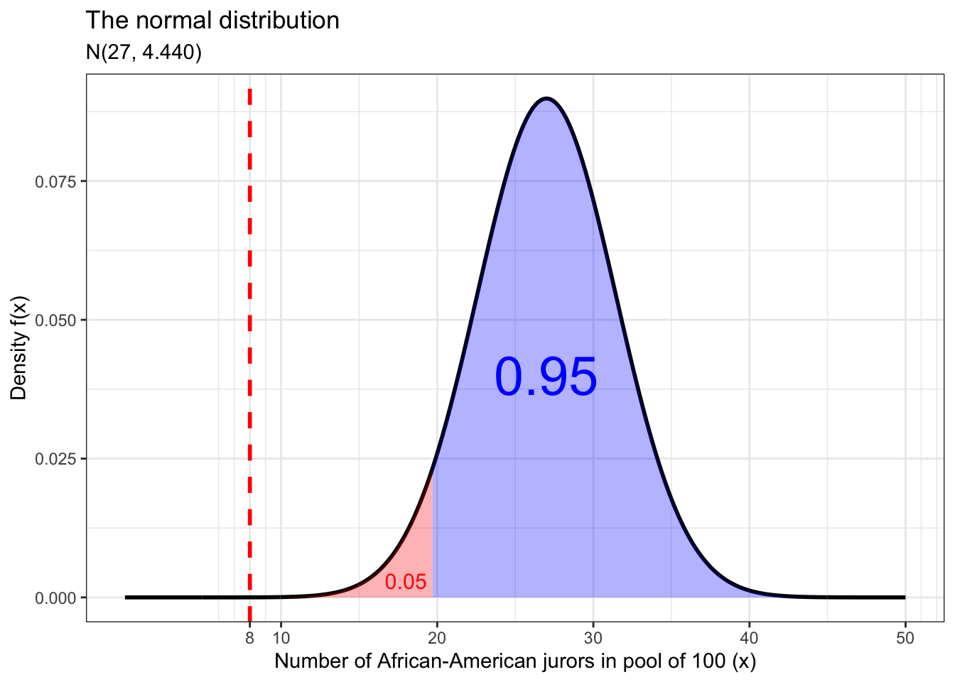
The last way we could test this hypothesis is through a process called bootstrapping, which we already did at the very beginning. Bootstrapping is when you resample from a single sample to generate a sampling distribution in order to draw inferences from it. The proportion of simulated jury pools with 8 or fewer African-American potential jurors is approximately equal to what the normal distribution predicts above. And the plot of the histogram with the vertical line drawn at x = 8 looks a lot like our normal distribution plot above. We can therefore use this information draw the same inferences. This is possible because of the central limit theorem.
##   eight_or_less_prop
## 1              1e-05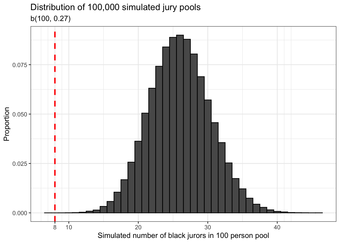
Have we shown that the Supreme Court of the United States committed a grave error in its decision? Not necessarily. But we have shown that there is some evidence of bias in jury pool formation in Talladega County for the trial of Robert Swain. At the very least we have shown that this issue is worthy of further investigation.