15 Tutorial 4: The Binomial Distribution
15.0.1 The binomial distribution in R
R has several built-in functions for the binomial distribution. They’re listed in a table below along with brief descriptions of what each one does.
| Binomial function | What it does |
|---|---|
dbinom(x, size, prob) |
P(X = x), the probability that X = x |
pbinom(q, size, prob, lower.tail = TRUE) |
P(X =< q), the probability that X takes a value less than or equal to q |
rbinom(n, size, prob) |
Generates numbers which follow a binomial distribution with the given parameters |
Let’s try these functions out to see how they really work.
We’ll start with rbinom(), a function which randomly generates numbers which follow a binomial distribution with given parameters. For our first test of it, we’ll generate one observation (n = 1) of a sample of size 100 (size = 100) and a probability of success of 0.3 (prob = 0.3).
## [1] 28The result printed above is the number of successes in a single sample of size 100. The proportion of successes is not exactly equal to the one we used to generate the data, but it is close, and the larger the sample size gets, the closer that actual proportion will be to that theoretical proportion.
Now let’s do something a little more interesting. What does the binomial distribution look like? We can generate some data using rbinom() and plot it using ggplot2 to find out. We’re going to use the same sample size and probability of success for rbinom() as before, but we’re going to generate a lot more data in order to get a good idea of what this distribution is supposed to look like.
set.seed(10)
binomial_data <- rbinom(1000, 100, 0.3)
binomial_data <- as.data.frame(binomial_data)
names(binomial_data) <- c('data')

binomial_data %>% ggplot() +
  geom_histogram(aes(x = data,
                     y = stat(count / sum(count))),
                     color = 'black') +
  geom_vline(xintercept = 30,
             size = 1,
             linetype = 'dashed',
             color = 'red') +
  theme_bw() +
  labs(x = 'Number of successes in 100 trials',
       y = 'Proportion',
       title = '1000 samples of b(100, 0.3)')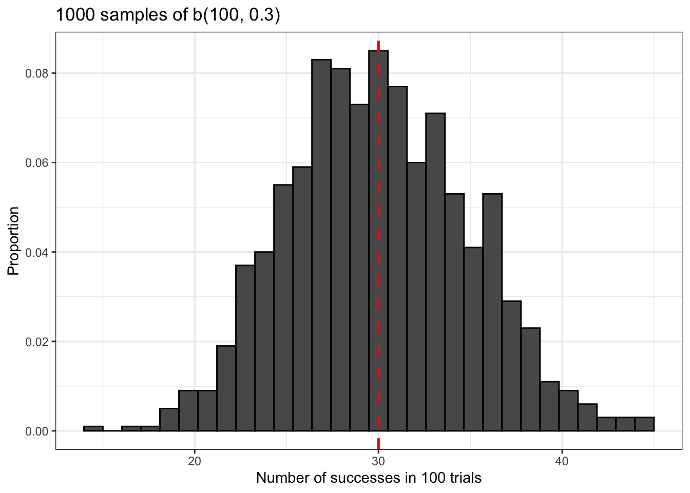
The binomial distribution is approximately normal. Notice also that it’s centered at the average of our distribution, np = 30. This is marked with a vertical red dashed line.
The next function we’re going to learn about is dbinom(), which gives the probability that a binomial variable with certain parameters takes a certain value. Let’s use it to calculate the probability that the variable we’ve been working with will take the average value np = 30.
## [1] 0.08678386The probability of this event is about 8.67%. But what does this really mean?
binomial_data %>% ggplot() +
  geom_histogram(aes(x = data,
                     y = stat(count / sum(count)),
                     fill = data == 30),
                 color = 'black') +
  theme_bw() +
  labs(x = 'Number of successes in 100 trials',
       y = 'Proportion',
       title = '1000 samples of b(100, 0.3)')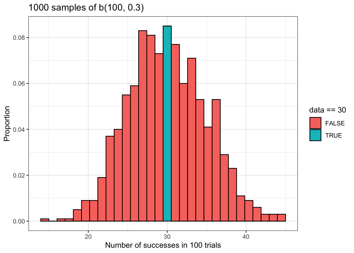
The plot above should make the probability we just calculated using dbinom() a bit clearer. Basically, this probability is given by the area inside of the turquoise bar. That bar represents all of the samples in binomial_data for which there were 30 successes. In other words, it represents all of the times that our random variable took a value of 30.
However, it is important to note that the probability we calculated using dbinom() is a theoretical probability that is not necessarily equal to the actual proportion of observations in our data that are equal to 30. We will calculate that empirical value below.
## [1] 0.08678386## proportion_of_30s
## 1 0.085The theoretical and empirical proportions are quite close, but they are not equal.
The next function we’re going to learn about is pbinom(), which is a cumulative probability function. It returns the probability that a random binomially distributed variable takes on a value that is less than or equal to a certain value. Let’s try it out.
## [1] 0.5491236The probability that our random variable will take a value less than or equal to the given value in the given sample size with a given probability of success is about 54%. The plot below illustrates this using our sample data.
binomial_data %>% ggplot() +
  geom_histogram(aes(x = data,
                     y = stat(count / sum(count)),
                     fill = data <= 30),
                 color = 'black') +
  theme_bw() +
  labs(x = 'Number of successes in 100 trials',
       y = 'Proportion',
       title = '1000 samples of b(100, 0.3)')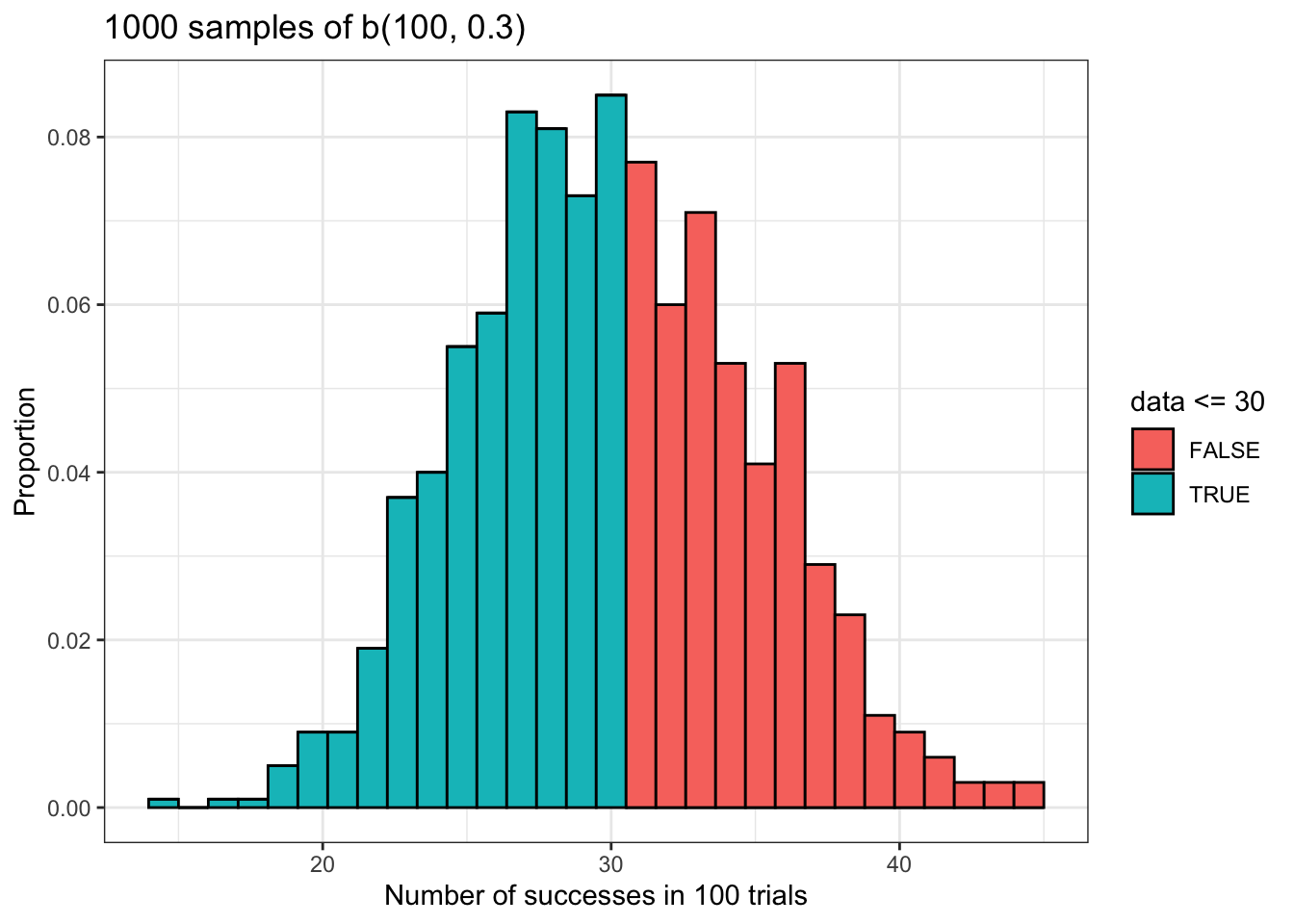
As we did with the dbinom() function, we’ll compare our theoretical and empirical cumulative probabilities. Once again, they’re close but not equal.
## [1] 0.5491236## less_than_or_equal_to_30
## 1 0.558We’re not finished with pbinom() yet. So far, we’ve only considered it for calculating a left tailed probability. What about a right tailed probability?
pbinom() has an optional argument called lower.tail, whose default value is TRUE, that we can use for calculating right tailed probabilities. It is also possible to calculate right tailed probabilities by writing 1 - pbinom(q, size, prob), but I think changing the value of the lower.tail argument is a better way to do this because it’s more immediately obvious what you’re trying to accomplish.
Now let’s try it for the complement of the left tail probability we just calculated above. We’ll also compare this to the proportion in our data and visualize this result.
## [1] 0.4508764## more_than_30
## 1 0.442binomial_data %>% ggplot() +
geom_histogram(aes(x = data,
y = stat(count / sum(count)),
fill = data > 30),
color = 'black') +
theme_bw() +
labs(x = 'Number of successes in 100 trials',
y = 'Proportion',
title = '1000 samples of b(100, 0.3)')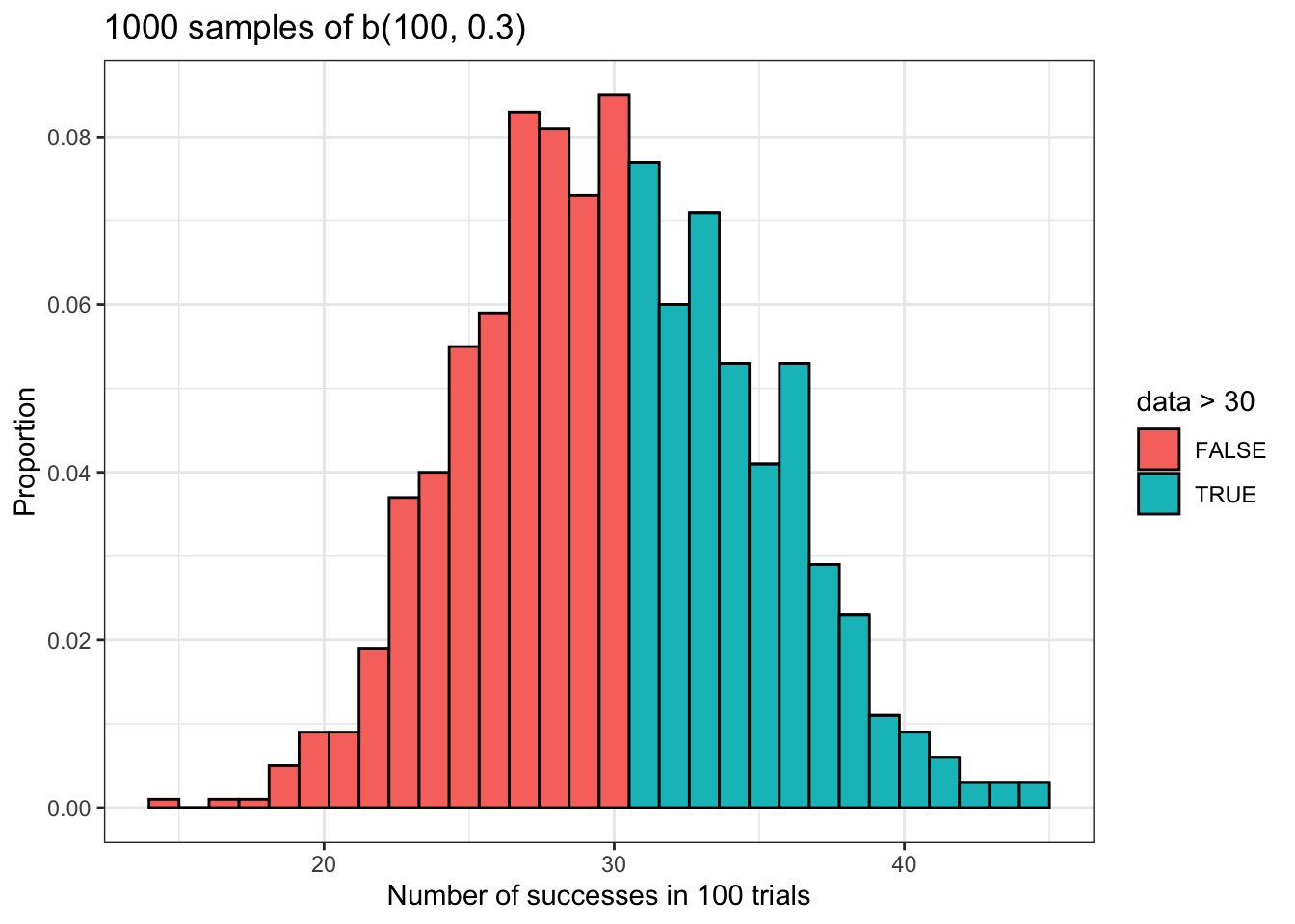
Here is something that is worth emphasizing: the value of lower.tail not only controls whether you are performing an left or right tailed test, but whether you are calculating the probability that a binomially distributed variable takes a value less than or equal to some value P(X <= x), or whether you are calculating the probability that a binomially distributed variable takes a value greater than but NOT equal to some value P(X > x). This is a bit subtle, but it is very important that you remember this in order to use these functions correctly.
15.0.2 Simulating flight overbooking using the binomial distribution
The following simulation is adapted from Probability with Applications in R by Robert Dobrow.
Every year, many people miss flights because they cancel at the last minute or are late to the airport. Research by Leder, et al. (2002) suggests that about 12% of airline passengers miss flights every year for these reasons.
This tendency for a significant percentage of passengers to miss their flights is well known among airlines. To deal with this, airlines typically overbook seats, meaning they sell more tickets for a flight than there are seats available because they can count on a significant percentage of passengers to fail to show up.
This is a somewhat risky strategy because there will be times when too many passengers show up and not all of them will be able to get seats. How often can we expect this to happen? We can use the binomial distribution to model an example.
Suppose that there is a flight with 100 seats, and 110 tickets have been sold. We’ll define “failing to show up on time for the flight” as a failure for this event, and we know the probability of this event is p = 0.12. As for a success, which would be “showing up on time for the flight”, the probability of this event is p = 1 - 0.12 = 0.88.
What is the probability that more than 100 passengers will show up on time for this flight? I.e., how likely is it that at least one too many people will show up for this flight and be unable to board because there isn’t any space? We can calculate this very quickly using pbinom().
## [1] 0.1366599This means there’s an approximately 13.5% chance that at least one too many people will show up on time for this flight and be unable to get a seat. This is intolerably high. What can airlines do to mitigate this risk? Let’s take a look at the relationship between the total number of seats sold and the probability that more than 100 people will show up for this flight on time. Let’s also assume that a typical airline can’t accept a probability of more than 5% that this will happen.
overbook_risks <- data.frame('Probability' = pbinom(100, 101:115, 0.88, lower.tail = FALSE),
                            'seats_sold' = 101:115)

overbook_risks %>% ggplot() +
  geom_line(aes(seats_sold,
                Probability),
            size = 1) +
  geom_hline(yintercept = 0.05,
             color = 'red',
             linetype = 'dashed',
             size = 0.25) +
  theme_bw() +
  labs(x = 'Seats sold',
       y = 'Probability of more than 100 people showing up on time',
       title = 'Overbooking risk for 100 passenger flight',
       subtitle = 'p = 0.88') +
  scale_x_continuous(breaks = seq(101, 115)) +
  scale_y_continuous(breaks = seq(0, 1, 0.05),
                     limits = c(0, 1))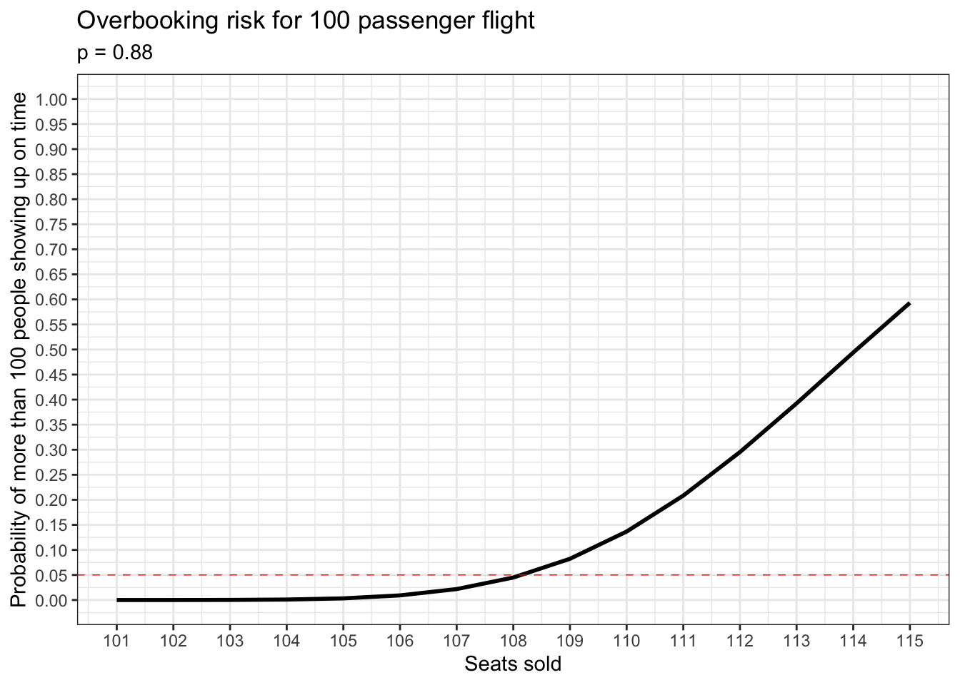
Judging from the plot above, it looks like the number of seats sold with the highest acceptable risk is 108.
##   Probability seats_sold
## 7  0.02184463        107
## 8  0.04492587        108
## 9  0.08231748        109
The probability of more than 100 people showing up on time if 108 seats are sold is about 4.5%. And this is the best we can do.
15.0.3 Simulating family composition in the United States using the binomial distribution
This simulation was adapted from the following lab which was given as part of a 2009 version of STAT 10 at UCLA.
http://www.stat.ucla.edu/~yexy/stat10/lab3.pdf
It is commonly believed that after conceiving a child, any given woman has an equal chance of giving birth to a boy or a girl. For many decades in the United States, this has not actually been true: about 51% of the babies born in the US every year are male. The article below summarizes a recent study with an interesting explanation for why this is. However, those reasons are well beyond the scope of our class.
The bit of information about this topic which concerns us is the popularity of female births. We can use the information about the popularity of male births to calculate the popularity of female births very easy: p = 1 - 0.51 = 0.49.
Suppose you have just gotten married and you and your spouse have decided to have three children. Suppose also that you want as many of these three children as possible to be girls. What are the probabilities for each number of girls that could join your family? We can use dbinom() to figure this out.
##   num_of_girls probability
## 1            0    0.132651
## 2            1    0.382347
## 3            2    0.367353
## 4            3    0.117649
It looks like the most likely outcome for your family is one girl. This is pretty disappointing given your preferences. How would this situation be different if girls were equally likely to be born as boys?
##   num_of_girls probability
## 1            0       0.125
## 2            1       0.375
## 3            2       0.375
## 4            3       0.125
In this situation you’re equally likely to have 1 or 2 girls. This is interesting to know, but it does not reflect reality.
So far we have only considered theoretical probabilities. Now we’re going to generate data to represent outcomes for other families of the same size and same preferences. Let’s start with 10 families.
set.seed(10)

dat_10 <- data.frame(dat = rbinom(10, 3, 0.49))

for (col in colnames(dat_10)){
  zero <- sum(dat_10[[col]] == 0) / length(dat_10[[col]])
  one <- sum(dat_10[[col]] == 1) / length(dat_10[[col]])
  two <- sum(dat_10[[col]] == 2) / length(dat_10[[col]])
  three <- sum(dat_10[[col]] == 3) / length(dat_10[[col]])

  column <- data.frame('prop_in_10_sims' = c(zero,
                                             one,
                                             two,
                                             three))
  family <- cbind(family, column)
}

family
## num_of_girls probability prop_in_10_sims
## 1 0 0.132651 0.1
## 2 1 0.382347 0.7
## 3 2 0.367353 0.2
## 4 3 0.117649 0.0Since the number of families is small, there’s a lot of random variation in our data. But the overall pattern matches our expectations from earlier when we were only thinking about theoretical probabilities. Notice that the most popular outcome from both theoretical and empirical standpoints is one girl per family.
Now let’s try this for 100 families.
set.seed(10)

dat_100 <- data.frame(dat = rbinom(100, 3, 0.49))

for (col in colnames(dat_100)){
  zero <- sum(dat_100[[col]] == 0) / length(dat_100[[col]])
  one <- sum(dat_100[[col]] == 1) / length(dat_100[[col]])
  two <- sum(dat_100[[col]] == 2) / length(dat_100[[col]])
  three <- sum(dat_100[[col]] == 3) / length(dat_100[[col]])

  column <- data.frame('prop_in_100_sims' = c(zero,
                                             one,
                                             two,
                                             three))
  family <- cbind(family, column)
}

family
## num_of_girls probability prop_in_10_sims prop_in_100_sims
## 1 0 0.132651 0.1 0.14
## 2 1 0.382347 0.7 0.47
## 3 2 0.367353 0.2 0.35
## 4 3 0.117649 0.0 0.04There is less variation in our simulated data for a larger number of families, but we still see the same basic pattern: one girl remains the most popular outcome among these families too.