10 Tutorial 2: Probability
10.0.1 Flipping a fair coin
Recall in discussion while we were reviewing section 1.1 of the Tanis/Hogg text we established definitions for the following two similar but not identical terms.
- Relative frequency: The proportion of times some event occurs during a certain number of trials
- n: Number of times a trial/experiment is run
- N(A): The number of times that event A occurs during n trials
- N(A)/n: Relative frequency of event A
- Probability: The proportion of times an event occurs when the number of trials is very large
- This is given by N(A)/n as n approaches infinity
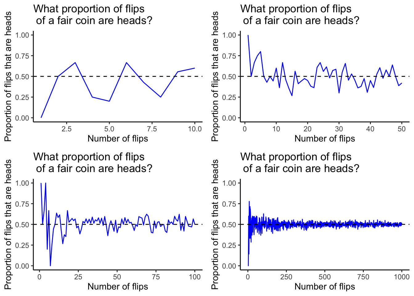
To illustrate these concepts, we looked at some plots which expand on an example that’s given in the textbook on page 5. The blue lines in each of the plots below represent the proportion of flips of a fair coin which are heads for a certain number of flips. The horizontal dashed line is drawn at the probability that any single flip of a fair coin will land on heads, which is 0.5.
Notice that as the number of flips increases, the proportion of flips that are heads converges towards the probability that a single flip of a fair coin will land on heads.

Now is a good time to introduce a couple of functions that are very valuable for running simulations like this.
10.0.2 Random and reproducible coin flips with sample() and set.seed()
Of course, if you want to run your own experiments with a fair coin, all you have to do is find one, start flipping and keep careful track of the result of each flip. For a small number of flips, say 10, this is pretty easy. But as the number of flips increases, it becomes much harder, mainly because flipping a coin over and over again, for hours or even days, is extremely boring and tedious. There has to be a better way!
Fortunately, R has powerful built-in functions for these sorts of activities. Repetitive tasks that would take practically forever if done manually instead take milliseconds. One of these is sample().
Before we can use sample() we need an object of some kind from which samples can be drawn. In this case we are flipping a coin, so this means that we need to create a coin inside of R. This has been done using a vector below and the object has been saved as coin.
sample() has two mandatory arguments. The first argument, x, is the object from which a sample is to be drawn and the second argument, size, is the size of the sample to be drawn. Let’s try drawing a sample of size 10 from coin. This is equivalent to flipping a real coin 10 times.
Unfortunately, if we try to draw 10 samples from coin, R will throw an error. This is because this function “cannot take a sample larger than the population when ‘replace = FALSE’”.
In this case the size of the population from which we are sampling is 2 because coin is a vector with 2 elements. The default value for the replace argument is FALSE, which means that by default sample() samples without replacement. In other words, when sample() draws at random from some population, it does not put back the elements from each individual sample. For coin, since there are only 2 elements in this vector, it’s not possible to sample from it without replacement 10 times because there will be no more elements to draw after the second draw.
Therefore in order to get sample() to draw 10 times from coin, we need to change the value of replace to TRUE.
##  [1] "Heads" "Tails" "Heads" "Heads" "Tails" "Heads" "Heads" "Heads"
##  [9] "Tails" "Tails"
The results of 10 flips of a fair coin are shown above. The form of this information is acceptable if you’re dealing with a small number of flips. But as the number of flips increases, this information will become increasingly difficult to interpret.
Since when we’re flipping a coin we are chiefly interested in how often the coin lands on each side, all we really need to know is the total number of times and/or the proportion of times this happens for each side. We already know a couple of pretty useful functions for doing this. Let’s try them for 100 flips of our coin.
##
## Heads Tails
## 502 498##
## Heads Tails
## 0.49 0.51Perhaps we would rather combine these results into a single table or dataframe of some kind.
freq <- as.vector(table(sample(coin, 100, replace = TRUE)))
prop <- prop.table(freq)
flips_df <- data.frame('Face' = coin,
                       'Frequency' = freq,
                       'Proportion' = prop)
flips_df
## Face Frequency Proportion
## 1 Heads 49 0.49
## 2 Tails 51 0.51There is one more detail about sample() that is very important for us to be aware of: its results are random. That is, every time you call the function, unless otherwise specified, the result will be different from the last time you called it. Sometimes this is exactly what you want, but other times you will want a random result that you generate to be reproducible by others. How can we make this happen?
Look back at the last three calls of sample() above. If you look closely at the results, you’ll notice that they are identical. This could be random, but it is exceedingly unlikely. And indeed it wasn’t, because in code that I have hidden I used a function called set.seed() to control the output of sample() in those three calls. The complete code for the summary dataframe we created above is below. The only difference is that there is one more line: set.seed(1).
set.seed(1)

freq <- as.vector(table(sample(coin, 100, replace = TRUE)))
prop <- prop.table(freq)
flips_df <- data.frame('Face' = coin,
                       'Frequency' = freq,
                       'Proportion' = prop)
flips_df
## Face Frequency Proportion
## 1 Heads 49 0.49
## 2 Tails 51 0.51For now, we only need to know two things about set.seed(). The first is the one and only argument that we will use with it, which is seed. This must be an integer.
Random processes like sample() in R are controlled by built in random number generation algorithms. When set.seed() is not used and a random process like sample() takes place, a seed integer is selected at random and unique values which correspond to this seed integer are produced each time the random process is conducted. In other words, when set.seed() is not used, a function like sample() will produce different results every time it is called.
freq_1 <- as.vector(table(sample(coin, 100, replace = TRUE)))
prop_1 <- prop.table(freq_1)
freq_2 <- as.vector(table(sample(coin, 100, replace = TRUE)))
prop_2 <- prop.table(freq_2)
two_coins <- data.frame('Face' = coin,
                        'Frequency_1' = freq_1,
                        'Proportion_1' = prop_1,
                        'Frequency_2' = freq_2,
                        'Proportion_2' = prop_2)
two_coins
## Face Frequency_1 Proportion_1 Frequency_2 Proportion_2
## 1 Heads 53 0.53 44 0.44
## 2 Tails 47 0.47 56 0.56We see an example of this above. Notice that there are different values for the frequencies/proportions of flips that came up heads or tails for the two coins. This happened because set.seed() was not used. Let’s see what happens if we use set.seed(1) on both calls of sample() in the code above.
set.seed(1)
freq_1 <- as.vector(table(sample(coin, 100, replace = TRUE)))
prop_1 <- prop.table(freq_1)
set.seed(1)
freq_2 <- as.vector(table(sample(coin, 100, replace = TRUE)))
prop_2 <- prop.table(freq_2)
two_coins <- data.frame('Face' = coin,
                        'Frequency_1' = freq_1,
                        'Proportion_1' = prop_1,
                        'Frequency_2' = freq_2,
                        'Proportion_2' = prop_2)
two_coins
## Face Frequency_1 Proportion_1 Frequency_2 Proportion_2
## 1 Heads 49 0.49 49 0.49
## 2 Tails 51 0.51 51 0.51Notice that when we use the same seed integer twice, we get the same output both times. This is because when the seed integer is fixed using set.seed() as it was above, the random number generation algorithm produces the values which correspond to that seed integer. In other words, since the seed integer is no longer random, the values produced by the random number generation algorithm are no longer random either. This is what we want to happen when we want to be able to reproduce the exact results of a certain simulated random process.
The second thing we need to know about set.seed() is that when you want to use it with a certain function like sample(), you have to call it together with that certain function every time. Look again at the code above. Notice that we called set.seed() twice. What happens if we only call it once?
set.seed(1)
freq_1 <- as.vector(table(sample(coin, 100, replace = TRUE)))
prop_1 <- prop.table(freq_1)
freq_2 <- as.vector(table(sample(coin, 100, replace = TRUE)))
prop_2 <- prop.table(freq_2)
two_coins <- data.frame('Face' = coin,
                        'Frequency_1' = freq_1,
                        'Proportion_1' = prop_1,
                        'Frequency_2' = freq_2,
                        'Proportion_2' = prop_2)
two_coins
## Face Frequency_1 Proportion_1 Frequency_2 Proportion_2
## 1 Heads 49 0.49 53 0.53
## 2 Tails 51 0.51 47 0.47The results of flipping our first coin are familiar, but the results for the second one are new. That is okay in this case, because that was what we were trying to show. But if we wanted to reproduce the results for the first coin with the second, we would have failed because we forgot to set the seed integer again.
10.0.3 Flipping an unfair coin
So far we have only considered a fair coin. What about an “unfair” coin?
To be clear, a fair coin is one for which the probability of landing on either side in a single given flip is equal. I.e., it’s a coin for which the probability of landing heads on a single flip is 0.5 and the probability of landing tails on a single flip is also 0.5.
An unfair or “biased” coin is one for which these probabilities are different. Do such coins exist? This is debatable. If you’re interested in learning a bit about this debate, follow the links below.
https://www.newscientist.com/article/dn1748-euro-coin-accused-of-unfair-flipping/
https://www.stat.berkeley.edu/~nolan/Papers/dice.pdf
Regardless of whether biased coins exist in reality, we can still use sample() to simulate what would happen if we did have one and we flipped it a certain number of times.
By default, sample() gives each element of the population from which it draws an equal probability of being drawn. A coin has two sides, and if there is an equal probability of landing on each side for any given single flip, then each side has a probability of 0.5. A die has six sides, and if there is an equal probability of landing on each side for any given single roll, then each side has a probability of about 0.1667. These are also the probabilities that sample() assigns by default.
sample() has a fourth optional argument, prob, which is a vector of numbers which can overwrite these default probabilities. The sum of elements in the vector must equal exactly 1 and each element must be non-negative.
Let’s try simulating 1,000 flips of a biased coin for which the probability of heads is 0.7 and the probability of tails is 0.3 and compare the outcome with that of a fair coin for the same number of flips.
set.seed(2)

fair_freq <- as.vector(table(sample(coin, 1000, replace = TRUE)))
fair_prop <- prop.table(freq)
biased <- c(0.7, 0.3)
biased_freq <- as.vector(table(sample(coin, 1000,
                                      replace = TRUE,
                                      prob = biased)))
biased_prop <- prop.table(biased_freq)
biased_df <- data.frame('Face' = coin,
                        'Fair_frequency' = fair_freq,
                        'Fair_proportion' = fair_prop,
                        'Biased_frequency' = biased_freq,
                        'Biased_proportion' = biased_prop)

biased_df
## Face Fair_frequency Fair_proportion Biased_frequency Biased_proportion
## 1 Heads 496 0.49 688 0.688
## 2 Tails 504 0.51 312 0.312Notice that the proportions of heads and tails for the fair coin are roughly equal, while these proportions for the biased coin are roughly equal to the biased proportions of 0.7 and 0.3 respectively.
10.0.4 Repeated sampling with replicate() and iteration with for loops
So far we’ve only learned how to take single random and reproducible samples using R. What if we want to sample the same population many times? We can use a function called replicate() for this.
replicate() has two mandatory arguments. The first, n, is the number of times you want to repeat some process that is paired with this function. The second argument, expr, is the process you want to repeat n times. Below is a basic example of a replicate() call and its output.
##       [,1]    [,2]    [,3]    [,4]    [,5]    [,6]    [,7]    [,8]
##  [1,] "Tails" "Heads" "Tails" "Tails" "Heads" "Heads" "Heads" "Heads"
##  [2,] "Tails" "Heads" "Tails" "Heads" "Tails" "Tails" "Heads" "Heads"
##  [3,] "Heads" "Tails" "Heads" "Tails" "Tails" "Tails" "Heads" "Tails"
##  [4,] "Tails" "Heads" "Heads" "Heads" "Tails" "Tails" "Tails" "Heads"
##  [5,] "Heads" "Heads" "Tails" "Tails" "Heads" "Tails" "Tails" "Heads"
##  [6,] "Tails" "Tails" "Tails" "Heads" "Tails" "Heads" "Heads" "Tails"
##  [7,] "Heads" "Tails" "Heads" "Heads" "Heads" "Tails" "Tails" "Tails"
##  [8,] "Tails" "Tails" "Tails" "Tails" "Tails" "Tails" "Heads" "Heads"
##  [9,] "Heads" "Heads" "Heads" "Heads" "Tails" "Tails" "Heads" "Tails"
## [10,] "Tails" "Tails" "Heads" "Tails" "Tails" "Heads" "Tails" "Tails"## [1] "matrix"Above we see the results of 8 seperate samples of 10 coin flips. Now instead of being limited to taking one sample of a certain size at a time, we can quickly produce many samples of a certain size at a time! Neat!
However, in its current form these results are not very useful because they are hard to summarize and visualize. Of course we could perform these tasks by hand, but if that were ideal, we would not be learning R programming. So what should we do?
The first thing we need to do is look at the type of data that replicate() produced here. It is an object of class matrix. If you’ve learned about matrix or linear algebra before, this type of mathematical object should be familiar to you. If not, that is not a problem here because we cannot use this object in its current form anyway, so we will turn it into a dataframe.
set.seed(8)

more_flips <- replicate(8, sample(coin, 10, replace = TRUE))

more_flips_df <- data.frame(more_flips)

colnames(more_flips_df) <- c('first',
                             'second',
                             'third',
                             'fourth',
                             'fifth',
                             'sixth',
                             'seventh',
                             'eighth')
more_flips_df
## first second third fourth fifth sixth seventh eighth
## 1 Tails Heads Tails Tails Heads Heads Heads Heads
## 2 Tails Heads Tails Heads Tails Tails Heads Heads
## 3 Heads Tails Heads Tails Tails Tails Heads Tails
## 4 Tails Heads Heads Heads Tails Tails Tails Heads
## 5 Heads Heads Tails Tails Heads Tails Tails Heads
## 6 Tails Tails Tails Heads Tails Heads Heads Tails
## 7 Heads Tails Heads Heads Heads Tails Tails Tails
## 8 Tails Tails Tails Tails Tails Tails Heads Heads
## 9 Heads Heads Heads Heads Tails Tails Heads Tails
## 10 Tails Tails Heads Tails Tails Heads Tails TailsNow our coin flip sample matrix is a coin flip dataframe with column names that are a bit more intuitive than before. However, there are some obvious improvements to be made. For one thing, we can’t tell at a glance how many heads and tails we got for each experiment with this coin. This means it’s time for more data cleaning.
The first stage of our data cleaning involves an interative process called a for loop. If you’ve taken an introductory Computer Science course before, you already know what this is, and you have probably used them to perform some repetitive operation over and over again and store the results inside of an appropriate data structure. In this case, that is still a dataframe.
clean_flips <- data.frame(matrix('', ncol = 3, nrow = 0))
# creating an empty dataframe to use with our for loop

colnames(clean_flips) <- c('flip', 'heads', 'tails')
#giving the columns of the empty dataframe appropriate names

for (col in names(more_flips_df)){
  heads <- sum(more_flips_df[[col]] == 'Heads')
  # adding up the number of heads in each column of more_flips_df
  tails <- sum(more_flips_df[[col]] == 'Tails')
  # adding up the number of tails in each column nof more_flips_df
  row_df <- data.frame('trial' = col,
                       'heads' = heads,
                       'tails' = tails)
  # inserting trial name, number of heads and number of tails
  # into an appropriate data structure
  clean_flips <- rbind(clean_flips, row_df)
  # adding the name, number of heads and number of tails to a row
  # of the blank dataframe
}

clean_flips
## trial heads tails
## 1 first 4 6
## 2 second 5 5
## 3 third 5 5
## 4 fourth 5 5
## 5 fifth 3 7
## 6 sixth 3 7
## 7 seventh 6 4
## 8 eighth 5 5Now our coin flip data is much cleaner. The notes inside of the code explain what each object is for and what each step of the for loop does. Thanks to this process, we can now tell at a glance how many heads and how many tails we got for each of the 8 trials we ran. This is a good way of summarizing this data.
However, although our data is cleaner, it is not yet tidy. The simplest defintion of “tidy data” that I have found comes from Hadley Wickham, author of one of the very first papers about this topic: “each variable is a column, each observation is a row, and each type of observational unit is a table”. In the last couple of tutorials we were already working with tidy data, although we may not have realized it. We need to put our data into tidy format so that we can use tidyverse packages on it such as ggplot2. Back to the drawing board!
But first, what would it mean for our data to be tidy in this specific situation?
For our data, each observation consists of three variables. The first is the number of the trial that was being run, the second is whether or not the result of an individual coin flip in that trial was heads and the third is whether or not the result in that trial was tails. The first is a factor variable and the last two are logical variables. This means that each row of our tidy dataset must look something like the printout below.
## [1] "fourth" "TRUE" "FALSE"Since we have three variables and we performed a total of 80 coin flips, we need to make a dataframe with three columns and 80 rows. Now let’s compile our tidy coin flip dataframe!
tidy_flips <- data.frame(matrix('', ncol = 3, nrow = 0))
colnames(tidy_flips) <- c('trial', 'heads', 'tails')
# blank dataframe for storing results of individual flips

for (col in names(more_flips_df)){
  row_df <- data.frame('trial' = col,
                  'heads' = more_flips_df[[col]] == 'Heads',
                  'tails' = more_flips_df[[col]] == 'Tails')
  # stores the trial name, whether the flip was heads and whether the
  # flip was tails for a single coin flip inside an appropriate
  # data structure
  tidy_flips <- rbind(tidy_flips, row_df)
  # pastes the result of a flip into a dataframe for all flip results
}

head(tidy_flips, 15)
## trial heads tails
## 1 first FALSE TRUE
## 2 first FALSE TRUE
## 3 first TRUE FALSE
## 4 first FALSE TRUE
## 5 first TRUE FALSE
## 6 first FALSE TRUE
## 7 first TRUE FALSE
## 8 first FALSE TRUE
## 9 first TRUE FALSE
## 10 first FALSE TRUE
## 11 second TRUE FALSE
## 12 second TRUE FALSE
## 13 second FALSE TRUE
## 14 second TRUE FALSE
## 15 second TRUE FALSE## [1] 80 3We did it! Our tidy dataframe rows look the way we wanted them to, and a quick check of this object’s dimensions using the dim() function shows that we indeed have 80 rows and 3 columns. This iteration process was a little different from the last one, and there are notes inside of the for loop which explain how it worked.
Now that our data is tidy, we can visualize it using ggplot2.
tidy_flips %>% ggplot(aes(x = trial, fill = heads)) +
  geom_bar(position = 'dodge', color = 'black') +
  theme_bw() +
  scale_fill_discrete(name = 'Coin face',
                      labels = c('Tails', 'Heads')) +
  labs(title = 'Results of 8 trials of 10 flips of a fair coin',
       x = 'Trial',
       y = 'Frequency')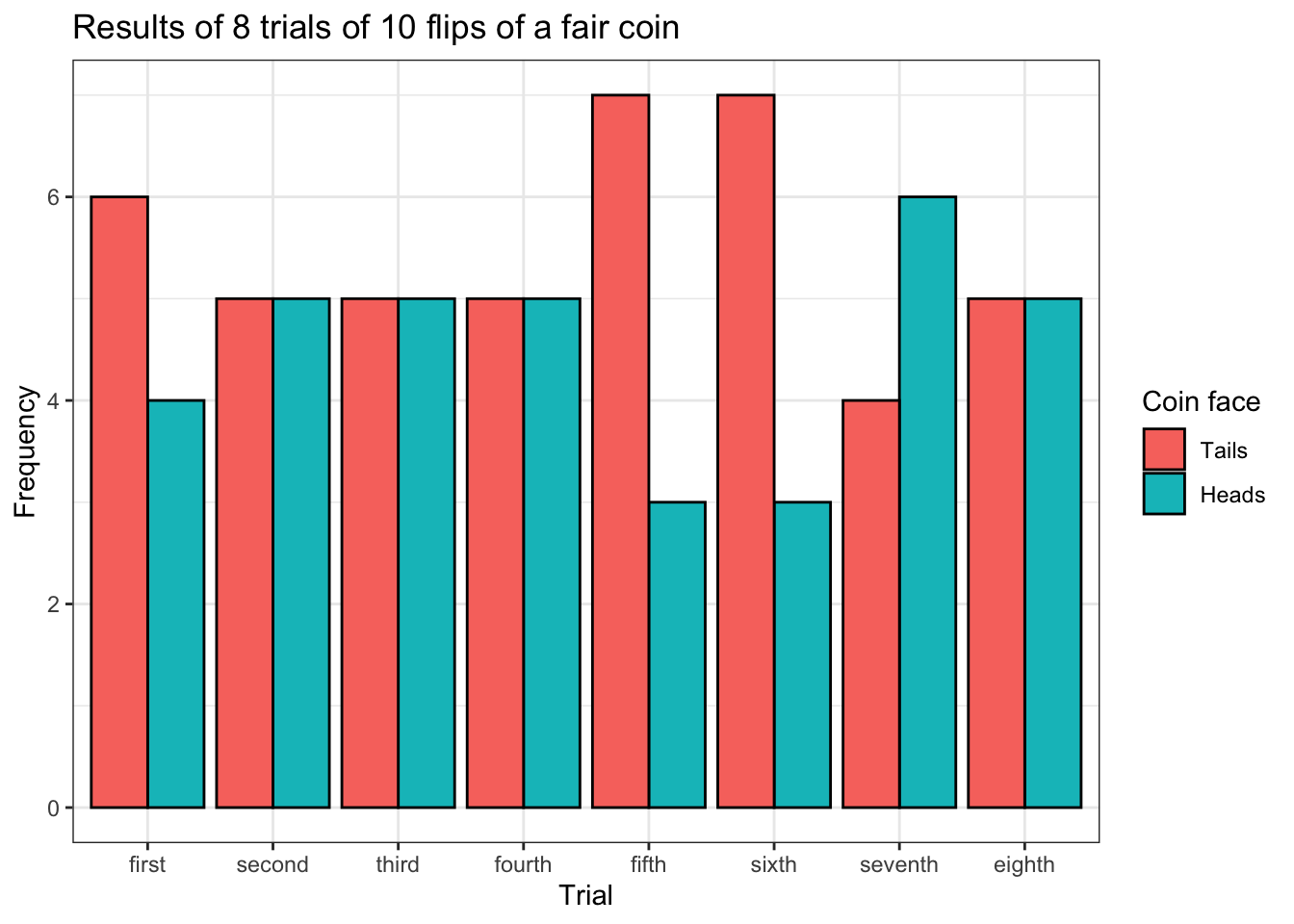
The graph above is an example of a grouped bar plot. Each pair of bars for each flip represents the number of heads and tails for each trial. But this plot is a bit crowded, which makes it hard to read, so this information is probably better presented in some other format.
tidy_flips %>% ggplot(aes(x = trial, fill = heads)) +
  geom_bar(position = 'fill', color = 'black') +
  theme_bw() +
  scale_fill_discrete(name = 'Coin face',
                      labels = c('Tails', 'Heads')) +
  labs(y = 'Proportion',
       title = 'Results of 8 trials of 10 flips of a fair coin')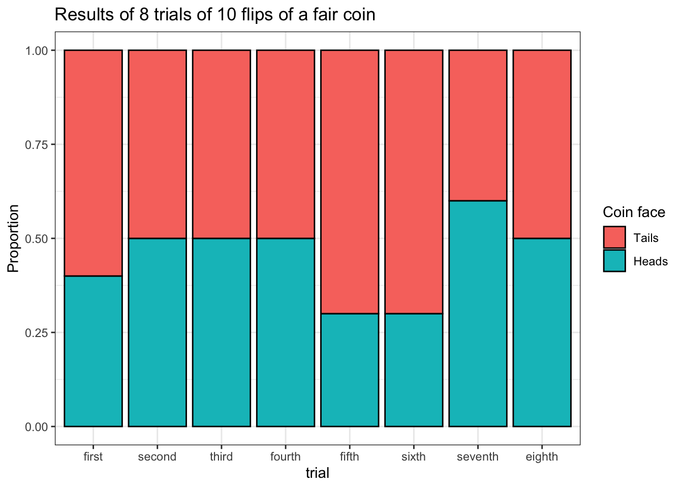
The above plot is of a familiar type and it is much easier to read.
10.0.5 Illustrating a principle of probability using functional programming
At the very beginning of this tutorial we saw a visualization which illustrated a mathematical principle of probability: as the number of times an experiment of an event with a given probability is performed increases, the proportion of times that event is a success converges to that probability. Here it is again below. In this case, these figures track the proportion of times a flipped coin lands on heads in more and more trials.
How can we show something like this ourselves for some other event? This will require functional programming. We’re going to do this for the biased coin we worked with earlier.
The first thing we need to do is create a function that will calculate the proportion of successes of some event with a certain probability. This begins with defining an object as a function with a single argument. Here we will define that argument as B for no particular reason. But for more complex functions it is important to give your arguments intuitive names.
flip_heads <- function(B){
  coin <- c('Heads', 'Tails')
  biased <- c(0.7, 0.3)
  flips <- replicate(B, sample(coin, 1,
                               replace = TRUE,
                               prob = biased))
  flips_df <- data.frame(flips)
  prop <- sum(flips_df$flip == "Heads") / length(flips_df$flip)
  return(prop)
}

list(flip_heads(10), flip_heads(50), flip_heads(100), flip_heads(1000))
## [[1]]
## [1] 0.8
##
## [[2]]
## [1] 0.74
##
## [[3]]
## [1] 0.7
##
## [[4]]
## [1] 0.709The first thing this function does is something familiar: it samples with replacement from a coin object B times and saves that as a local variable. After that, it changes that variable into a dataframe. Next, it calculates the proportion of flips inside of that dataframe that are heads. Finally, it returns that proportion. A few runs of the function show that it works.
Now we need to use this function to start generating data that we can use to plot. But how?
The first step involves using lapply(), one of the members of the apply() family, which are some special functions for iteration in R. lapply() has two mandatory arguments.
The first argument is a list or vector of objects on which you want to run some function. In this case we’re going to try computing the proportion of flips which land on heads for 1, 2, 3, 4 and 5 flips. To make this easier to type and generalize inside of a function later, we’re going to use seq(1, 5) instead of writing the numbers out individually inside of a vector or list. The second argument is the function on which we want to run a given vector or list. In this case, it’s the function we just wrote, flip_heads(). Let’s give it a try.
## [[1]]
## [1] 0
##
## [[2]]
## [1] 0.5
##
## [[3]]
## [1] 0.6666667
##
## [[4]]
## [1] 0.5
##
## [[5]]
## [1] 1## [1] "list"The form of the result is familiar even though its output is unique.
Another thing we need to know about lapply() is the kind of output it produces. Our result is a list object, which is not a form of tidy data. Let’s get tidying!
set.seed(1)

lst <- lapply(seq(1, 5), flip_heads)
df <- ldply(lst, data.frame)
names(df) <- c('prop')

df$n <- seq(1, length(df$prop))

df
## prop n
## 1 1.0000000 1
## 2 1.0000000 2
## 3 0.3333333 3
## 4 0.7500000 4
## 5 0.8000000 5## [1] "data.frame"The first thing we need to do is split our list that gets generated by lapply() and run data.frame() over it. To do this, we have to use a different function, ldply(), because this will return a dataframe instead of another list. We’re also going to add another column, n, to keep track of the number of flips we’re making in each trial. This will be our x variable when we plot this data.
Now we have a tidy little dataframe, so we can plot our data using ggplot2.
df %>% ggplot(aes(x = n, y = prop)) +
  geom_line(color = 'red') +
  geom_hline(yintercept = 0.7,
             linetype = 'dashed') +
  theme_bw() +
  labs(x = 'Number of flips',
       y = 'Proportion of flips that are heads',
       title = 'What proportion of flips of a fair coin are heads?') +
  xlim(1, 5) +
  ylim(0, 1)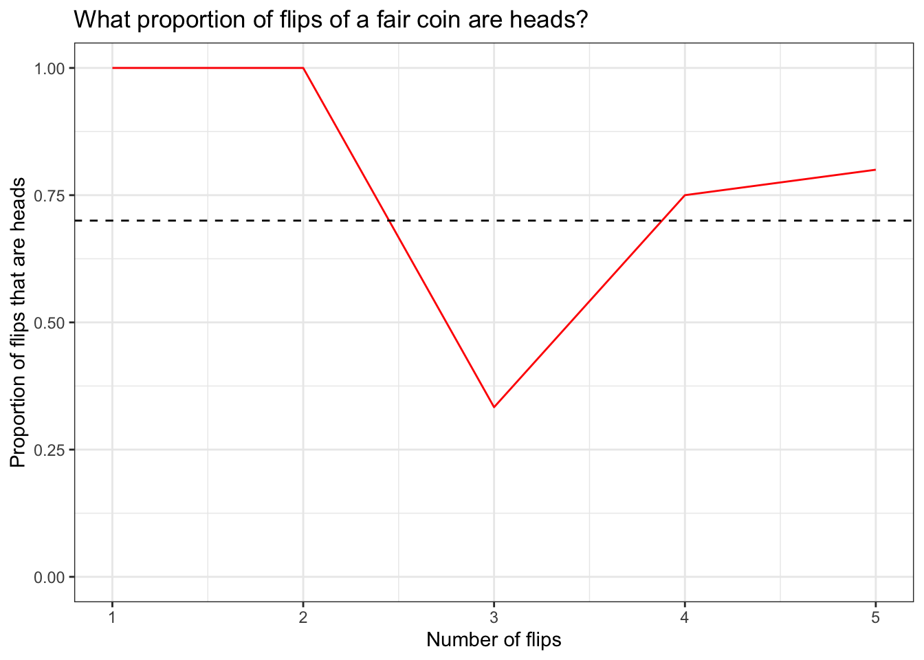
So far, so good. The last thing for us to do is take the function we wrote and the cleaning code, and put this stuff together with the plot we just made.
flip_heads <- function(B){
  # inserting the flip_heads function from before
  flip_heads <- function(B){
  coin <- c('Heads', 'Tails')
  biased <- c(0.7, 0.3)
  flips <- replicate(B, sample(coin, 1,
                               replace = TRUE,
                               prob = biased))
  flips_df <- data.frame(flips)
  prop <- sum(flips_df$flip == "Heads") / length(flips_df$flip)
  return(prop)
  }

  # data cleaning
  lst <- lapply(seq(1, B), flip_heads)
  df <- ldply(lst, data.frame)
  names(df) <- c('prop')
  df$n <- seq(1, length(df$prop))

  # data plotting
  ggplot(df, aes(x = n, y = prop)) +
  geom_line(color = 'red') +
  geom_hline(yintercept = 0.7,
             linetype = 'dashed') +
  theme_bw() +
  labs(x = 'Number of flips',
       y = 'Proportion of flips that are heads',
       title = 'What proportion of flips\n of a biased coin are heads?') +
  xlim(1, B) +
  ylim(0, 1)
}

set.seed(1)

ggarrange(flip_heads(5), flip_heads(10), flip_heads(100), flip_heads(1000))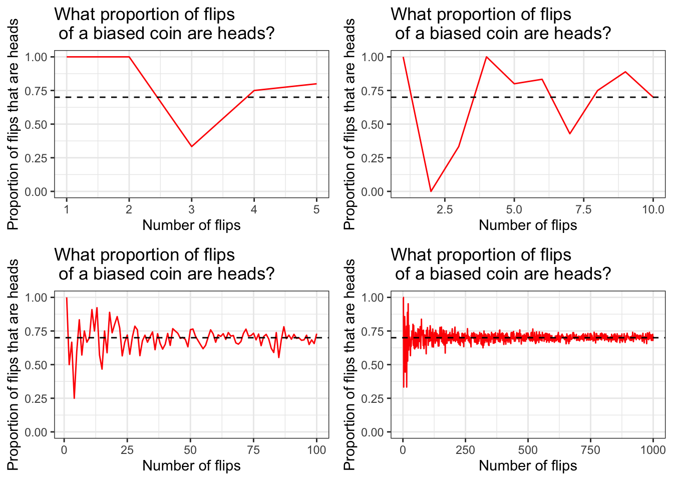
Great! Notice the position of the horizontal dashed line in each plot. It’s drawn at y = 0.7 because 0.7 is the probability of flipping heads with our biased coin.
10.0.6 More resources
You may remember the name “Hadley Wickham” from the DataCamp courses on functional programming in R. Dr. Wickham is a very influential figure in the field of statistical programming and he recently won one of the biggest awards in the field of Statistics for his work. A short article about that is linked below, along with a link to a page on his website which contains his big paper about tidy data.
https://www.nzherald.co.nz/nz/news/article.cfm?c_id=1&objectid=12254723
http://vita.had.co.nz/papers/tidy-data.html
Otherwise, if you find yourself struggling to complete any part of the lab which follows this tutorial, my advice is to use Google to try to find ways to overcome those problems. Practically every question that a student in this class could ask has already been answered, so all you really need to do is figure out how to adapt answers to similar questions to your specific situation. You can also try re-reading this tutorial and looking more closely at the example code that it contains.