19 Lab 5: The Poisson Distribution

19.0.1 Introduction

These days it is typical for militaries to pay substantial compensation to the survivors of a service member who is killed in combat or in certain service zones. For example, in the United States, the next of kin of a service member who is killed in combat or in a certain service zone is entitled to a $100,000 payment called a death gratuity. Other countries have similar systems in place which pay varying amounts depending on circumstances. Basic information about the American death gratuity system is linked below.

https://militarypay.defense.gov/Benefits/Death-Gratuity/

For the purpose of our lab, we’re going to make several assumptions that may not be historically accurate but will not affect the results of our analysis anyway.

First, we will assume that in 19th century Prussia, there was a death gratuity system like that in the USA which pays a fixed amount of money to the survivors of soldiers killed regardless of the circumstances of their deaths. This means that the family of a soldier killed while fighting valiantly in battle on his way to Paris receives the same amount as one who was kicked to death by a horse.

Second, although the name and metallurgical composition of the currency used in Prussia changed multiple times throughout the 19th century, we will pretend that they used only one currency called the thaler.

Third, we will assume that the size of the death gratuity for a Prussian soldier during the relevant period was 250 thaler and that this amount was worth about twice the median income in Prussia at the time, so it represents a considerable sum.

19.0.2 Your tasks

This simulation is based on the data about horse kick deaths among Prussian cavalry soldiers studied by Ladislaus Bortkiewicz.

Reproduce the summary dataframe below. Do this for 10,000 corps years instead of just 200. Use a seed integer of 12. Explain your results.

##   kick_deaths simulated_total theoretical_total
## 1           0            5412           5433.51
## 2           1            3262           3314.44
## 3           2            1075           1010.90
## 4           3             210            205.55
## 5           4              37             31.35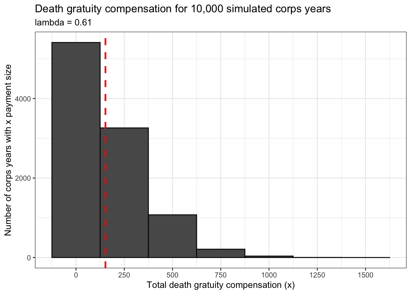
## 6          5+               4              4.25

Using your simulation data (not your summary data), reproduce the table and the visualization below. The dashed red line should be drawn at the average payment size.

## total_compensation
##    0  250  500  750 1000 1250 1500 
## 5412 3262 1075  210   37    3    1