12 Tutorial 3: Conditional Probability
12.0.1 The inspiration for this assignment
This tutorial and the lab which accompanies it was adapted from a STAT 13 lab that was given as part of a 2004 version of that course at UCLA. The original lab is linked below, though that file could disappear at any time because the instructor on whose webspace it’s hosted has not been at UCLA for a long time and they are not listed on the Statistics department’s faculty page.
http://www.stat.ucla.edu/~cocteau/teaching/stat13/labs/lab3.pdf
12.0.2 Our data
The dataset we will be working with is about spam email. We will not be working with the messages themselves, but rather a table of information about characteristics of over 4,500 email messages collected by researchers at Hewlett-Packard (HP) Labs. Some of these messages were spam and some were not. The original data is available at the link below.
https://archive.ics.uci.edu/ml/datasets/spambase
Our dataset differs from the original dataset hosted by UCI in some significant ways because of the cleaning process that it underwent to prepare it for this lab assignment. That process and its aims will be detailed in a subsequent tutorial.
Let’s have a peek at our data.
## 'data.frame':    4601 obs. of  49 variables:
##  $ make      : logi  FALSE TRUE TRUE FALSE FALSE FALSE ...
##  $ address   : logi  TRUE TRUE FALSE FALSE FALSE FALSE ...
##  $ all       : logi  TRUE TRUE TRUE FALSE FALSE FALSE ...
##  $ 3d        : logi  FALSE FALSE FALSE FALSE FALSE FALSE ...
##  $ our       : logi  TRUE TRUE TRUE TRUE TRUE TRUE ...
##  $ over      : logi  FALSE TRUE TRUE FALSE FALSE FALSE ...
##  $ remove    : logi  FALSE TRUE TRUE TRUE TRUE FALSE ...
##  $ internet  : logi  FALSE TRUE TRUE TRUE TRUE TRUE ...
##  $ order     : logi  FALSE FALSE TRUE TRUE TRUE FALSE ...
##  $ mail      : logi  FALSE TRUE TRUE TRUE TRUE FALSE ...
##  $ receive   : logi  FALSE TRUE TRUE TRUE TRUE FALSE ...
##  $ will      : logi  TRUE TRUE TRUE TRUE TRUE FALSE ...
##  $ people    : logi  FALSE TRUE TRUE TRUE TRUE FALSE ...
##  $ report    : logi  FALSE TRUE FALSE FALSE FALSE FALSE ...
##  $ addresses : logi  FALSE TRUE TRUE FALSE FALSE FALSE ...
##  $ free      : logi  TRUE TRUE TRUE TRUE TRUE FALSE ...
##  $ business  : logi  FALSE TRUE TRUE FALSE FALSE FALSE ...
##  $ email     : logi  TRUE TRUE TRUE FALSE FALSE FALSE ...
##  $ you       : logi  TRUE TRUE TRUE TRUE TRUE FALSE ...
##  $ credit    : logi  FALSE FALSE TRUE FALSE FALSE FALSE ...
##  $ your      : logi  TRUE TRUE TRUE TRUE TRUE FALSE ...
##  $ font      : logi  FALSE FALSE FALSE FALSE FALSE FALSE ...
##  $ 000       : logi  FALSE TRUE TRUE FALSE FALSE FALSE ...
##  $ money     : logi  FALSE TRUE TRUE FALSE FALSE FALSE ...
##  $ hp        : logi  FALSE FALSE FALSE FALSE FALSE FALSE ...
##  $ hpl       : logi  FALSE FALSE FALSE FALSE FALSE FALSE ...
##  $ george    : logi  FALSE FALSE FALSE FALSE FALSE FALSE ...
##  $ 650       : logi  FALSE FALSE FALSE FALSE FALSE FALSE ...
##  $ lab       : logi  FALSE FALSE FALSE FALSE FALSE FALSE ...
##  $ labs      : logi  FALSE FALSE FALSE FALSE FALSE FALSE ...
##  $ telnet    : logi  FALSE FALSE FALSE FALSE FALSE FALSE ...
##  $ 857       : logi  FALSE FALSE FALSE FALSE FALSE FALSE ...
##  $ data      : logi  FALSE FALSE FALSE FALSE FALSE FALSE ...
##  $ 415       : logi  FALSE FALSE FALSE FALSE FALSE FALSE ...
##  $ 85        : logi  FALSE FALSE FALSE FALSE FALSE FALSE ...
##  $ technology: logi  FALSE FALSE FALSE FALSE FALSE FALSE ...
##  $ 1999      : logi  FALSE TRUE FALSE FALSE FALSE FALSE ...
##  $ parts     : logi  FALSE FALSE FALSE FALSE FALSE FALSE ...
##  $ pm        : logi  FALSE FALSE FALSE FALSE FALSE FALSE ...
##  $ direct    : logi  FALSE FALSE TRUE FALSE FALSE FALSE ...
##  $ cs        : logi  FALSE FALSE FALSE FALSE FALSE FALSE ...
##  $ meeting   : logi  FALSE FALSE FALSE FALSE FALSE FALSE ...
##  $ original  : logi  FALSE FALSE TRUE FALSE FALSE FALSE ...
##  $ project   : logi  FALSE FALSE FALSE FALSE FALSE FALSE ...
##  $ re        : logi  FALSE FALSE TRUE FALSE FALSE FALSE ...
##  $ edu       : logi  FALSE FALSE TRUE FALSE FALSE FALSE ...
##  $ table     : logi  FALSE FALSE FALSE FALSE FALSE FALSE ...
##  $ conference: logi  FALSE FALSE FALSE FALSE FALSE FALSE ...
##  $ spam      : logi  TRUE TRUE TRUE TRUE TRUE TRUE ...
We see that we have and 4,601 observations in this dataset. Each observation represents one email message.
There are 49 variables in this dataset. The first 48 variables represent whether or not a word was present in a message. For example, if the value for will is TRUE for an observation, this means that the word “true” was present in this email message. If the value for business is FALSE for an observation, this means that the word “business” was not present in that email message.
The 49th variable, spam, represents whether or not an observation is a spam message. A value of TRUE means it is a spam message and a value of FALSE means that it is not a spam message. How many spam messages and how many real messages are in this dataset?
## spam
## FALSE  TRUE   Sum
##  2788  1813  4601
Notice that the table above looks a little bit different from ones we’ve made in the past. By now you’ve probably developed strong enough analytical skills to understand why, so I will leave that up to you. This tutorial will contain more examples of tables like this.
12.0.3 Which words did each message contain?
Since each observation consists of 49 different logical variables, we need to come up with a creative way of browsing this data. One preliminary question worth asking is, which words in the dataset were present in the 25th message?
An easy way we could try to answer this is by using bracketing. To get the 25th row of our dataset, all we have to type into our console is email2[25, ]. This will return the 25th row and all of the values for every column. And we’ll add [1:48] on the end because for now we only care about which words were present in an email message and not whether it was spam or not.
##     make address   all    3d   our  over remove internet order  mail
## 25 FALSE   FALSE FALSE FALSE FALSE FALSE  FALSE    FALSE FALSE FALSE
##    receive  will people report addresses  free business email   you credit
## 25   FALSE FALSE  FALSE  FALSE     FALSE FALSE    FALSE FALSE FALSE  FALSE
##     your  font   000 money    hp   hpl george   650   lab  labs telnet
## 25 FALSE FALSE FALSE FALSE FALSE FALSE  FALSE FALSE FALSE FALSE  FALSE
##      857  data   415    85 technology  1999 parts    pm direct    cs
## 25 FALSE FALSE FALSE FALSE      FALSE FALSE FALSE FALSE  FALSE FALSE
##    meeting original project   re   edu table conference
## 25   FALSE    FALSE   FALSE TRUE FALSE FALSE      FALSE
This output is not very easy to interpret. Sure, it prints out every word that’s present in the dataset along with whether these words were present or not in the 25th message. But it’s hard to tell at a glance which words were present and which weren’t, and it’s even hard to tell the difference between the words and their truth values because the words and truth values are both words. There has to be a better way! And indeed there is: through functional programming.
Below is a function called email_words() that I wrote to answer this question more effectively. If you’ve learned about flow statements (if/else statements) in a Computer Science class before, the flow statement in this function may look redundant to you. This is due to a certain idiosyncrasy in the R language that’s way beyond the scope of this discussion. But if you ever find yourself trying to use flow statements together with for loops inside of R, this is something that you’ll need to read up on in order to get these things to work together.
Anyway, let’s try using this function and see what it does.
email_words <- function(data, row){
  email_words_list <- c()
  for (i in 1:48){
    if(isTRUE((data[row,][i] != 0))){
      email_words_list <- c(email_words_list, colnames(data)[i])
    }
  }
  return(email_words_list)
}

email_words(email2, 25)
## [1] "re"It looks like the only word that was present in the 25th observation was "re". This is likely the automatically generated “Re:” heading that email clients use to indicate that a message is a reply to an earlier message.
Let’s try using this function one more time for the 250th message and see if we can get a more interesting result.
##  [1] "all"     "our"     "remove"  "order"   "mail"    "receive" "free"
##  [8] "email"   "you"     "hp"      "1999"    "direct"
This observation contained many more words than the 25th observation.
12.0.4 Filtering and re-ordering data with dplyr
It’s nice that we’ve figured out a quick way of checking to see which words were present in each of the 4,601 messages, but it would be more interesting to see which words are most popular in real messages and which are most popular in spam messages. We can do that by filtering and then re-ordering our data.
First, we’re going to create two new dataframes. One will contain only spam messages and the other will contain only real messages.
This is only the first step. By now we ought to know without looking that spam_messages and real_messages look just like email2 because all we did above was split that email2 object into two objects based on whether or not the value for spam was TRUE or FALSE for each observation in that dataset. Both of these smaller datasets have 49 variables, but a fraction of the observations of the original dataset.
Since we want to rank the counts of each of the words in spam_messages and real_messages, we need to generate a summary dataframe which contains this information. We will do that below using a familiar process. First we generate seperate summaries for the spam messages and the real messages and then we paste these summaries together side by side using cbind(). Finally, we’ll have a look at our work so far using head().
spam_summary <- data.frame(matrix(nrow = 0, ncol = 2))

real_summary <- data.frame(matrix(nrow = 0, ncol = 2))

for (col in colnames(spam_messages[1:48])){
  count <- sum(spam_messages[[col]])
  row <- data.frame('spam word' = col, 'spam count' = count)
  spam_summary <- rbind(spam_summary, row)
}

for (col in colnames(real_messages[1:48])){
  count <- sum(real_messages[[col]])
  row <- data.frame('real word' = col, 'real count' = count)
  real_summary <- rbind(real_summary, row)
}

big_summary <- cbind(spam_summary, real_summary)

head(big_summary)
## spam.word spam.count real.word real.count
## 1 make 641 make 412
## 2 address 625 address 273
## 3 all 1115 all 773
## 4 3d 39 3d 8
## 5 our 1134 our 614
## 6 over 681 over 318We are making good progress. Now we have a table which shows the frequencies of each of the words in messages that are real and in messages that are spam. But we need to reorder this information by count to get what we’re really looking for.
top_10_spam_words <- spam_summary %>% arrange(desc(spam.count)) %>% head(10)

top_10_real_words <- real_summary %>% arrange(desc(real.count)) %>% head(10)

small_summary <- cbind(top_10_spam_words, top_10_real_words)

small_summary
## spam.word spam.count real.word real.count
## 1 you 1608 you 1619
## 2 your 1466 will 1182
## 3 will 1143 hp 1040
## 4 our 1134 your 957
## 5 all 1115 re 824
## 6 free 989 hpl 784
## 7 mail 827 all 773
## 8 remove 764 george 772
## 9 business 697 1999 728
## 10 email 688 our 614It looks like there is some overlap between the 10 most popular words in real and spam messages. For example, the most popular word for both types of messages is "you"! But there are some differences. For instance, the word free is one of the top spam words and the word hp is one of the top real words.
Another question worth asking is which words have the biggest difference in frequency between spam and real messages. I.e., if we subtract the frequencies of each spam word and each real word, which ones have the biggest differences in frequency?
big_summary$spam_minus_real <- big_summary$spam.count - big_summary$real.count

big_summary %>% arrange(desc(spam_minus_real)) %>% select(spam.word, spam_minus_real) %>% head(5)
## spam.word spam_minus_real
## 1 free 737
## 2 remove 721
## 3 money 627
## 4 000 525
## 5 our 520The spam words with the biggest differences in frequency are shown above. It’s not hard to imagine why these would appear more frequently in spam messages, especially words like “free” and “money”.
##   real.word spam_minus_real
## 1        hp            -990
## 2    george            -764
## 3       hpl            -757
## 4      1999            -627
## 5      labs            -433
The real words with the biggest differences in frequency are shown above. Their frequenies have a negative sign because they appeared in far more real messages than spam messages. It’s a bit tricker to imagine why this would be so, but when you think about where our data came from, it becomes clearer.
12.0.5 Using proportion tables for conditional probability calculations
So far we’ve only looked at which words were most common in spam and real messages and compared their frequencies. This is not the same thing as calculating or comparing the probabilities of events related to these words.
Now that we’ve covered the concept of conditional probability in class, now would be an appropriate time to use it. But before we proceed, recall the definition of conditional probability.
Conditional probability: The conditional probability of one event given that some other event has happened. (Defined mathematically below.)
- P(A|B) = P(A and B) / P(B)
It is also possible to calculate conditional probabilities using Bayes’ formula, but we will be using the above definition of conditional probability instead because it’s easier to work with on our programming tasks.
Recall that P(A and B) is the probability that events A and B occur simultaneously. It is also known as the intersection of A and B.
Now we’re going to have a look at a table which can be used to represent marginal probabilities (defined in a moment) and the probabilities of two events.
basic_table <- addmargins(prop.table(table(email2$credit,
                                           email2$spam,
                                           dnn = c('credit', 'spam'))))

basic_table
## spam
## credit FALSE TRUE Sum
## FALSE 0.59574006 0.31210606 0.90784612
## TRUE 0.01021517 0.08193871 0.09215388
## Sum 0.60595523 0.39404477 1.00000000This table shows two variables: spam and credit. There are four events in this table, one for each TRUE and FALSE value of the spam and credit variables. (By the way, you make a table like this, you should use the addmargins() function and the dnn parameter. If you don’t, it will make your table very difficult to read.)
The marginal probabilities of each event is given in the bottom row and the rightmost column. For example, the probability that spam is TRUE is 0.39404477 and the probability that credit is FALSE is 0.90784612.
The probabilities of intersection are given by cells which represent the simultaneous occurrence of two different events. For example, the probability that credit is TRUE and spam is TRUE at the same time is 0.08193871.
basic_table is a table object, and so we can extract elements from it using bracketing like we sometimes do with dataframes. For instance, I can extract and print the intersectional probability I identified above by using bracketing. The numbers I will use correspond to the row and column where that probability is located. This is easy to figure out because it’s the same basic coordinate system we use when graphing things in the first quadrant of a 2D space. And this is something that you’ll need to remember in order to complete your lab.
## [1] 0.08193871Now let’s try to do something interesting with this table. Let’s answer this question: What is the probability that a message is spam given that it contains the word ‘credit’?
First, let’s make sure we understand the question in terms of probability. A big clue here is the use of the word ‘given’. This means that we’re trying to calculate this kind of probability: P(A|B). But which event is which? Recall that P(A|B) in plain English is “the probability of event A given event B”. This means that for the question we’re trying to answer, event A is spam == TRUE and event B is credit == TRUE. We need to use this formula: P(A|B) = P(A and B) / P(B).
We’re going to find the answer in a programmatic way.
##        spam
## credit       FALSE       TRUE        Sum
##   FALSE 0.59574006 0.31210606 0.90784612
##   TRUE  0.01021517 0.08193871 0.09215388
## Sum 0.60595523 0.39404477 1.00000000## [1] 0.8891509This is a pretty interesting finding: if a message in our dataset contains the word ‘credit’, there is an approximately 89% chance that this message is spam. This strongly suggests that blocking all messages that contain this word is a good idea.
Now what about the probability that a message is spam given that the message does not contain the word ‘credit’? You may be tempted to blurt out that it’s the complement of the result above, but you’d be incorrect. We need to use the conditional probability formula again in order to get the correct answer.
##        spam
## credit       FALSE       TRUE        Sum
##   FALSE 0.59574006 0.31210606 0.90784612
##   TRUE  0.01021517 0.08193871 0.09215388
## Sum 0.60595523 0.39404477 1.00000000## [1] 0.3437874This probability is more than triple the complement of the last result, but this result is still consistent with our last one: it’s more likely than not that if a message contains the word ‘credit’, it is a spam message.
12.0.6 Using functional programming to rapidly calculate many conditional probabilities
Now we’re going to narrow our focus on one conditional probability for each word in our dataset: the probability that a message is spam given that it contains a certain word.
In the background I’ve written a function called p_spam_given_word() which can calculate this probability for any of the words in our dataset. Below we see a familiar result.
## [1] 0.8891509By itself this function isn’t very powerful, although it significantly simplifies the process of calculating individual conditional probabilities for each of the words in our dataset. This function becomes much more powerful when we use it together with other tools we’ve learned how to use in previous labs and tutorials.
Suppose we wanted to calculate the probability that a message is spam given it contains each of the words in our dataset. We could run p_spam_given_word() 48 more times, once for each word in our dataset, and that would give us each of the individual probabilities that we need, and that should only require one or two lines of code if we really know what we’re doing.
Then if we’re really clever, we can figure out a way to store this information in a way that will allow us run a slightly deeper analysis on it. For instance, we could divide the words up by their probabilities into groups that are high, medium and low risk for being spam given that each one is present in a message.
##     Min.  1st Qu.   Median     Mean  3rd Qu.     Max.
## 0.006757 0.090839 0.468764 0.426424 0.701489 0.946716
Since these probabilities range from about 0 to about 100%, a good way to group them would be to create groups for words with probabilities that range from 0%-33% another for 33%-66% and another for 66%-100%.
And finally, if we’re really, really smart, we ought to be able to take this dataset and summarize it visually because that would make our work truly meaningful since we’re so great at creating slick visualizations now.
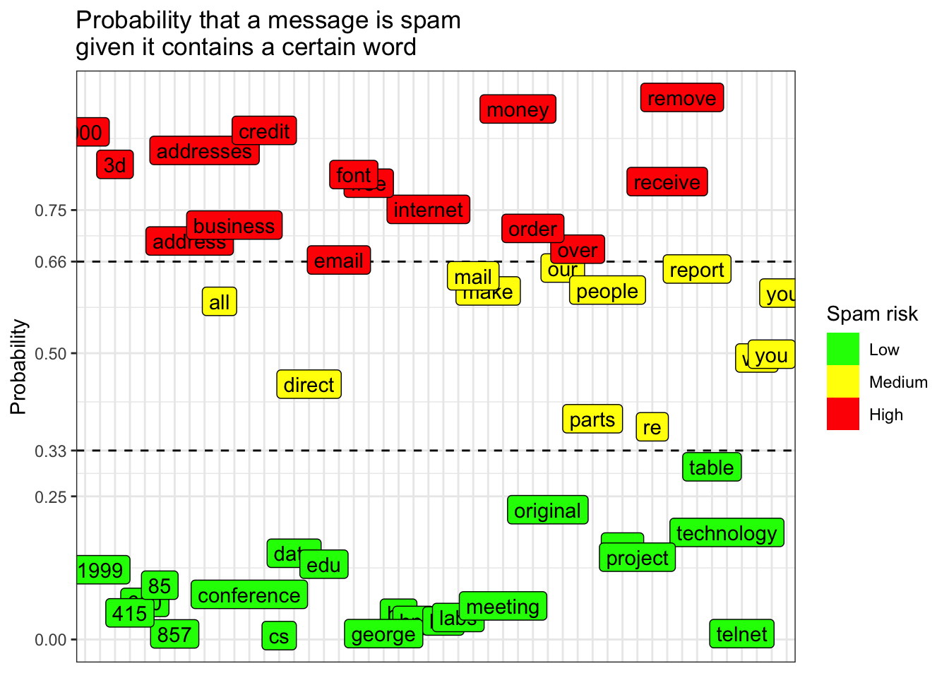
We can definitely reproduce the plot above! But it will take some research and experimentation…