18 Tutorial 5: The Poisson Distribution
18.0.1 The Poisson distribution in R
R has several built-in functions for the Poisson distribution. They’re listed in a table below along with brief descriptions of what each one does.
| Poisson function | What it does |
|---|---|
dpois(x, lambda) |
P(X = x), the probability that there will be x successes per period for an event with an average number of lambda successes |
ppois(x, lambda, lower.tail = TRUE) |
P(X <= x), the cumulative probability that there will be x or fewer successes per period for an event with an average number of lambda successes. Returns P(X > x), the cumulative probability that there will be more than x successes per period for the same variable when lower.tail = FALSE. |
rpois(n, lambda) |
Returns n randomly generated numbers that follow a Poisson distributionn with an average number of lambda successes |
We will begin our demom with rpois(). First we’ll use it to make one (n = 1) randomly generated observation of a random variable that follows the Poisson distribution and has an average number of 10 successes (lambda = 10) per period.
## [1] 8This single observation isn’t very interesting on its own because there’s nothing we can say about it that hasn’t already been said.
The first somewhat interesting thing we’ll do with rpois() is generate some data that we can use to plot this distribution so we can see what it looks like. We’re going to generate 1,000 random observations with the same value for lambda.
set.seed(2)

poisson_data <- data.frame('data' = rpois(1000, 10))

poisson_data %>% ggplot() +
  geom_histogram(aes(x = data,
                     y = stat(count / sum(count))),
                     color = 'black',
                 binwidth = 1) +
  geom_vline(xintercept = 10,
             size = 1,
             linetype = 'dashed',
             color = 'red') +
  theme_bw() +
  labs(x = 'Number of successes per period',
       y = 'Proportion',
       title = '1,000 samples of Pois(lambda = 10)')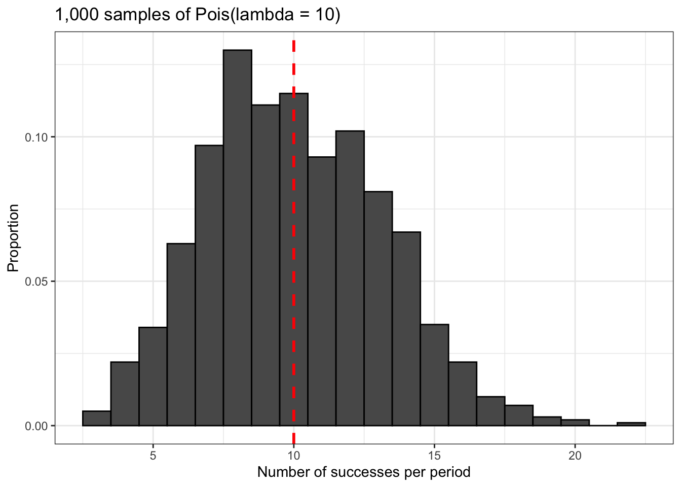
dpois() and ppois() work the same way as their counterparts from the binomial distribution. We’ll see them in action in the following practical examples.
18.0.2 Predicting the number of babies born in a hospital
The following question was taken from Probability in with Applications in R by Robert Dobrow.
Data from the maternity ward in a certain hospital shows that there is a historical average of 4.5 babies born in this hospital every day. What is the probability that 6 babies will be born in this hospital tomorrow?
First, let’s calculate the theoretical probability of this event using dpois(). The number of successes we’re considering is 6, so we will set x = 6. Additionally, this historical average of 4.5 babies per day is our value for lambda, so we will set lambda = 6.
## [1] 0.1281201The theoretical probability of 6 babies being born tomorrow if the historical average is 4.5 is about 13%.
Now let’s try simulating births in this hospital for a year (n = 365) using rpois() and compare the proportion of days in which there were 6 births to the theoretical probability we calculated above. We will also visualize this result.
set.seed(2)

babies <- data.frame('data' = rpois(365, 4.5))

babies %>% ggplot() +
  geom_histogram(aes(x = data,
                     y = stat(count / sum(count)),
                     fill = data == 6),
                 binwidth = 1,
                 color = 'black',) +
  scale_x_continuous(breaks = 0:10) +
  labs(x = 'Number of babies born per period',
       y = 'Proportion',
       title = '365 simulated births in a hospital with Pois(lambda = 4.5)') +
  theme_bw()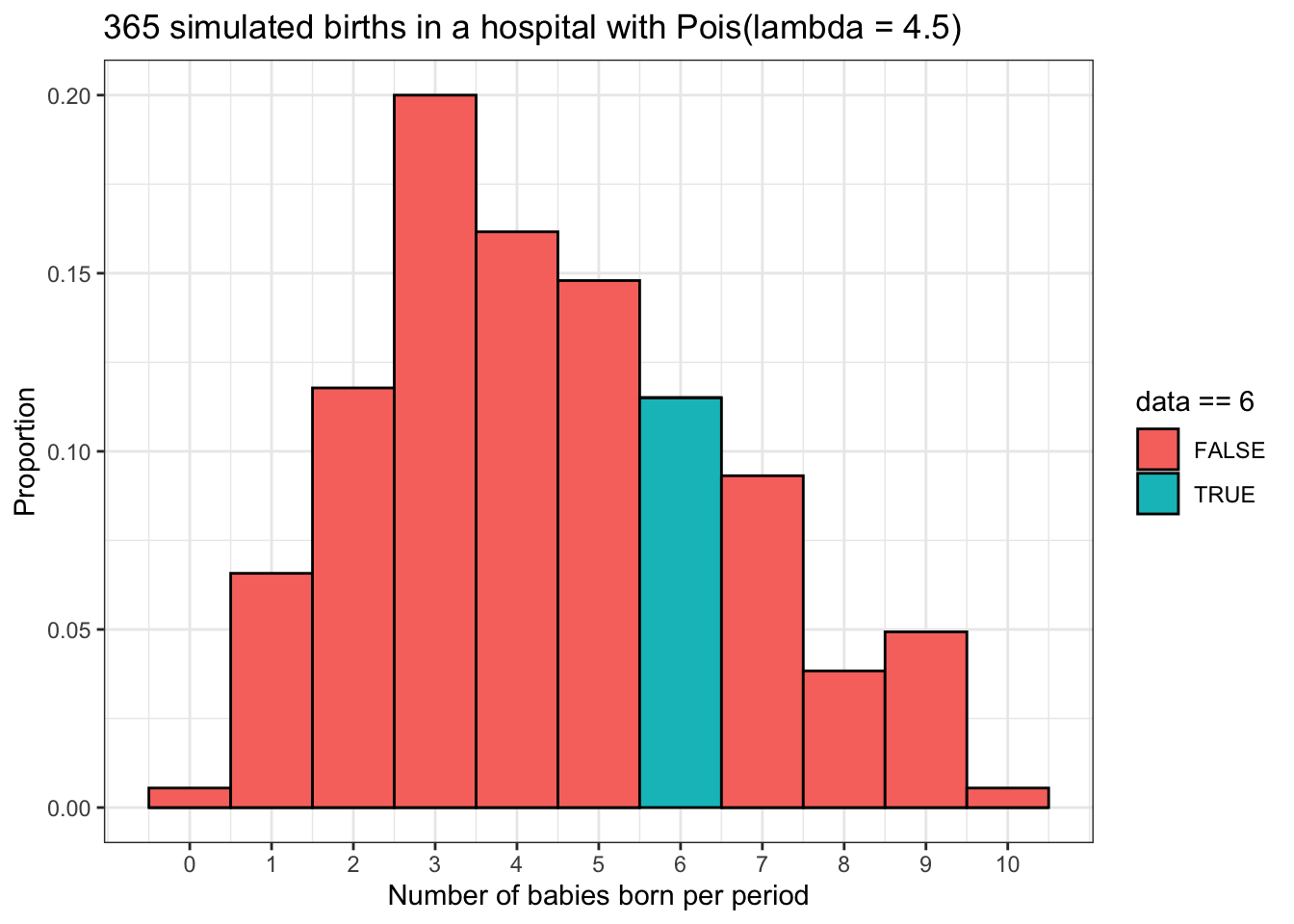
##   six_babies
## 1  0.1150685
The simulated result of about 11.5% is pretty close to our theoretical probability of about 13%.
What about the probability of more than 6 babies being born?
## [1] 0.1689494This theoretical probability is about 16.9%. Remember that cumulative probability functions in R calculate P(X > x) when lower.tail = FALSE. Here it calculated P(X > 6) = P(X >= 7).
What about the corresponding proportion in our simulation?
babies %>% ggplot() +
  geom_histogram(aes(x = data,
                     y = stat(count / sum(count)),
                     fill = data > 6),
                 binwidth = 1,
                 color = 'black',) +
  scale_x_continuous(breaks = 0:10) +
  labs(x = 'Number of babies born per period',
       y = 'Proportion',
       title = '365 simulated births in a hospital with Pois(lambda = 4.5)') +
  theme_bw()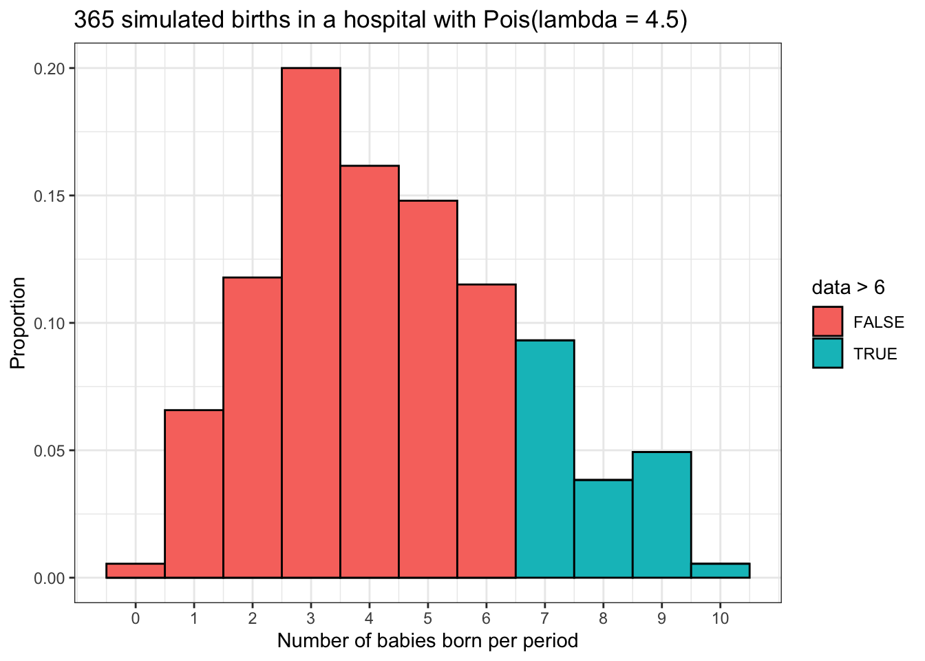
##   six_babies
## 1  0.1863014
The simulated proportion of about 18.6% is pretty close to the theoretical proportion we calculated above.
18.0.3 Simulating deaths by horse kick of Prussian cavalry soldiers
The data for this simulation comes from Probability in with Applications in R by Robert Dobrow.
One of the most famous studies based on the Poisson distribution was by Ladislaus Bortkiewicz, a Polish economist and statistician, in his book The Law of Small Numbers. This book actually contained two studies: one about deaths by horse kicks of Prussian cavalry soldiers and one about child suicides in Prussia. The former is far better known than the latter, probably because its topic is far less grim. The results of his horse kicking death study are still used to teach students about the Poisson distribution today, and our class will be no exception.
In his study, Bortkiewicz considered 20 years of data for 10 corps (groups) of Prussian cavalry soldiers. Over this period there were 122 total deaths by horse kick among these soldiers. Bortkiewicz divided the data into 20 individual periods for each group of soldiers, for a total of 20 x 10 = 200 corps years. The average number of deaths by horse kick was 121 / 200 = 0.61, which means that lambda = 0.61. The data from his study is shown below.
##   num_deaths observed poisson_probability expected
## 1          0      109               0.543    108.7
## 2          1       65               0.331     66.3
## 3          2       22               0.101     20.2
## 4          3        3               0.021      4.1
## 5          4        1               0.003      0.6
## 6         5+        0               0.000      0.0
The first column of the table, num_deaths, gives values for the number of horse kick deaths per corps year. This means that for 109 corps years, there were no horse kick deaths. poisson_probabilty tells us the theoretical probability of such an event according to the Poisson distribution. Death by horse kick is pretty rare even among people who spend lots of time around horses (like 19th century Prussian cavalry soldiers for instance), so the Poisson distribution predicts that most of the time this won’t happen, which is why 0 deaths has the highest theoretical probability of all the events.
The expected column tells us the total number of deaths in 200 corps years that the Poisson distribution predicts when lambda = 0.61. It is given by multiplying the theoretical probability of each number of deaths per corp year by 200, the total number of corps years. For example, the Poisson distribution predicts that there will be 0 deaths in 108.7 of 200 corps years. Notice how this number of total expected deaths for all corps years, along with all the other estimations, is very close to what was actually observed. This is why Bortkiewicz believed that deaths by horse kick among the Prussian cavalry soldiers he studied followed a Poisson distribution.
18.0.4 Simulating costs of car accidents
The following question was taken from Probability in with Applications in R by Robert Dobrow.
Suppose that the number of accidents per month at a busy intersection in the center of a certain city is 7.5. This event follows a Poisson distribution and lambda = 7.5.
Every time an accident occurs at this intersection, the city government has to pay about $25,000 to clean up the area. What is the average cost of these accidents per year?
This question is a lot easier than it probably sounds. We know that the average number of accidents per month is 7.5. We also know that there are 12 months in a year, so the average number of accidents per year is just the product of these two numbers. Finally, since we also know the average cost per accident, the average cost of accident clean-up per year for this city is just the product of these three numbers.
## [1] 2250000In a typical year, this city can expect to pay about $2.25 million in accident clean-up costs for this intersection.
One thing that we should remember, however, is that we are talking about a random variable which follows a certain distribution. This means that there will always be some random variation in annual accident costs for this city. To get an idea of how much accident costs can vary, we’re going to run a simulation.
First, we’ll simulate the annual accident cost for one year. We’ll use n = 12 because lambda = 7.5 represents the average number of accidents per month, and we want to simulate 12 months. We will save these results as a variable called accidents.
Next, we’ll multiply each element inside of accidents by 25,000 in order to calculate the average cost per month of accident clean-up. Finally, we will add these monthly costs together to get the total annual cost.
## [1] 2325000In this simulation, the total cost of cleaning up after accidents was about $2.32 million.
Now we’re going to use replicate() to simulate accident costs at this intersection for 1,000 years. We’re using a high number so that we can get a good look at what this distribution looks like.
set.seed(2)

cost_sim <- data.frame('data' = replicate(1000, sum(25000 * rpois(12, 7.5))))

cost_sim %>% ggplot() +
  geom_histogram(aes(x = data,
                     y = stat(count / sum(count))),
                 color = 'black',
                 binwidth = 100000) +
  geom_vline(xintercept = mean(cost_sim$data),
             color = 'red',
             size = 1,
             linetype = 'dashed') +
  scale_x_continuous(breaks = c(1500000,
                                2000000,
                                2259225,
                                2500000,
                                2500000,
                                3000000)) +
  labs(x = 'Annual accident cost',
       y = 'Proportion',
       title = 'Distribution of 1,000 simulated years of car accident costs',
       subtitle = 'Pois(lambda = 7.5)') +
  theme_bw()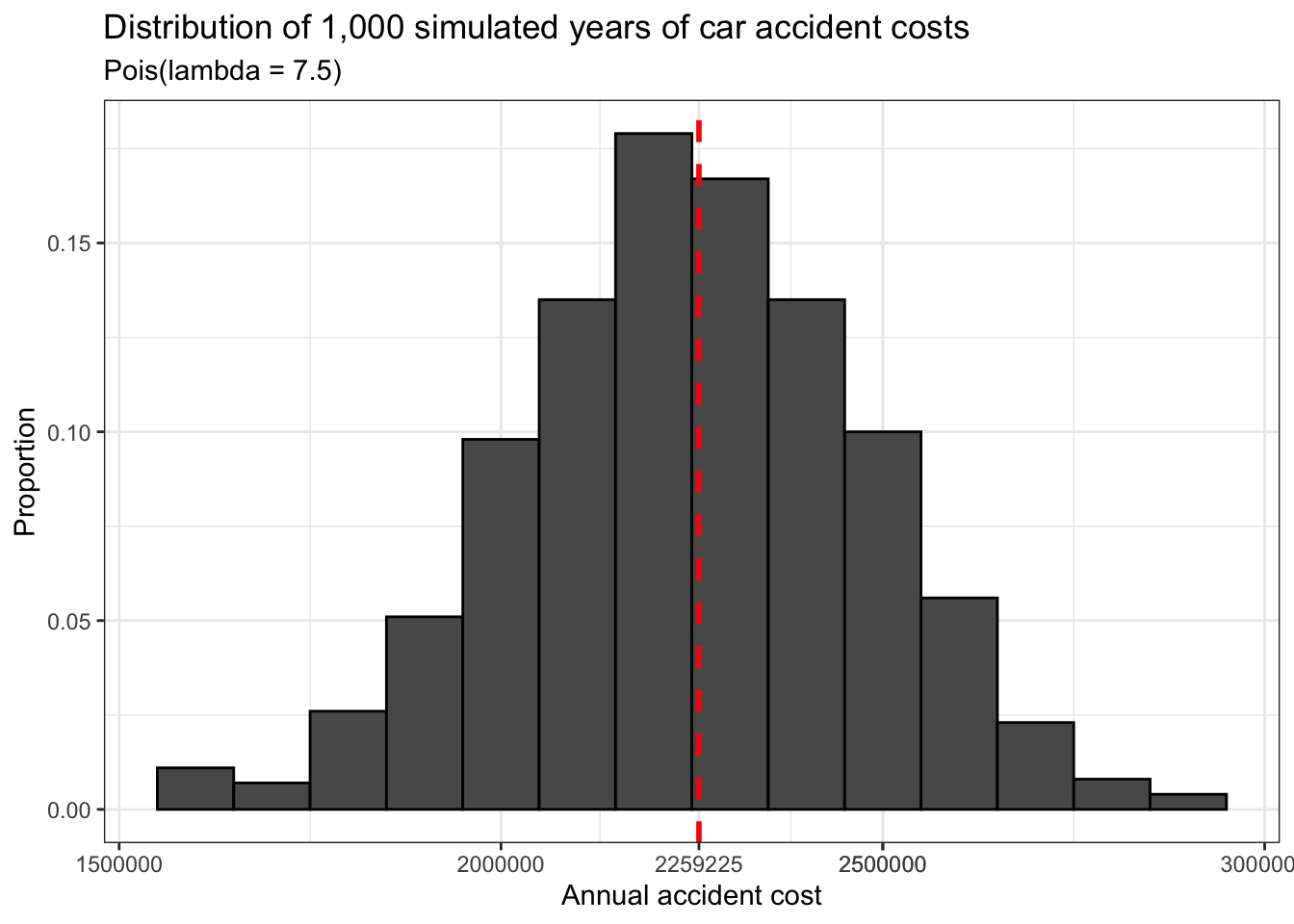
## [1] 2259225In this simulation, the mean cost of accident clean-up is about $2.26 million, which is quite close to the theoretical total. This cost is marked on the histogram above with a dashed red line.
How big is this town? Is this the most dangerous intersection in terms of accident frequency? How does it compare to others in the town? Unfortunately we can’t answer any of these questions. But spending over $2 million in a typical year to deal with accidents at a single intersection is a sign that something needs to be done about the design of that intersection to decrease the frequency of those accidents because at the very least, they are a drain on the city’s finances.
18.0.5 Bomb hits over London during World War 2
The following two paragraphs are copied directly from Probability with Applications in R by Robert Dobrow.
The following setting is very general. Suppose
nballs are thrown inton / lambdabowls so that each ball has an equal chance of landing in any bowl. If a ball lands in a bowl, call it a “hit.” The chance that a ball hits a particular bowl is 1 / (n / lambda) =lambda / n. Keeping track of whether or not each ball hits that bowl, the successive hits form a Bernoulli sequence, and the number of hits has a binomial distribution with parameters n andlambda / n. Ifnis large, the number of balls in each bowl is approximated by a Poisson distribution with parametern * (lambda / n) = lambda.
Many diverse applications can be fit into this ball and bowl setting. In his classic analysis of Nazi bombing raids on London during World War II, William Feller (1968) modeled bomb hits (balls) using a Poisson distribution. The city was divided into 576 small areas (bowls) of 1/4 km squared. The number of areas hit exactly
ktimes was counted. There were a total of 537 hits, so the average number of hits per area was 537/576 = 0.9323.
The data from this study is shown in the table below.
##   hits observed_hits expected_hits
## 1    0           229        226.70
## 2    1           211        211.40
## 3    2            93         98.60
## 4    3            35         30.67
## 5    4             7          7.10
## 6   5+             1          1.60
This table is interpreted in a way similar to the one about horse kicking deaths. The first column represents the number of balls (bombs) that landed in one of the bowls (1/4 km square areas). The second and third columns represent the number of areas in which a certain number of bombs landed and the number of areas in which it was expected that number of bombs would land according to the Poisson distribution, respectively. Like the study about horse kick deaths, the observed and expected values are quite close because the random variable being examined appears to follow a Poisson distribution.
While I was looking around the internet to find more information about this dataset and possibly the original data itself, I stumbled upon some important historical details about this study that are worth knowing about so that we properly understand what this data really tells us.
Dobrow’s description of this study’s history contains a couple of minor factual errors. William Feller was not the original author of the London bombing study. He did write about it in his 1968 book An Introduction to Probability Theory and Its Applications, Vol. 1, but the passage which covers this topic contains a citation for a 1946 article in an actuarial journal by a different author, R. D. Clarke. This article is linked below.
https://www.actuaries.org.uk/system/files/documents/pdf/0481.pdf
Also, this data doesn’t cover all of London, but rather only a 144 square kilometer section of the southern part. This is explained in the original article linked above.
Finally, the original purpose of the study was to investigate whether or not bombs that were dropped on this part of London landed in clusters or not. That is, were the patterns in which the bombs landed in this part of the city random or not? As the author of the original study explains in his short article, the answer is that there is insufficient evidence to conclude that the bombs landed in clusters as was frequently claimed.
Now we’re going to run a simulation with this data that’s based on one by Robert Dobrow. His original script for this simulation is linked below.
https://people.carleton.edu/~rdobrow/Probability/R%20Scripts/Chapter%203/Balls.R
The first thing we’re going to do is create some variables which match the ones described in the quotes from Dobrow at the beginning of this section. n will represent the number of bombs (balls) dropped on this section of London and u will represent the number of 1/4 square kilometer sections of the city that were subject to bombing (bowls). We will assume n is sufficiently large to define lambda = n / u. The bowls variable is a vector of length u in which each element (bowl) represents one quarter square kilometer section of the city that was subject to bombing. Each element (bowl) is initialized with a value of 0 because before the bombing starts, 0 bombs have landed in each section (bowl).
We will use a for loop for this simulation. The loop iterates through a sequence of numbers from 1 to n = 537, once for each bomb that was dropped in the section of London that was targeted. The first line of the loop selects one number at random from a sequence of numbers from 1 to u = 576. (Remember that all of these numbers have starting values of 0.) The number that is selected represents the section of the city where the bomb will land. The second line of the loop increases the number of bombs that have landed on this part of the city by 1 to indicate that a bomb has landed there during this round of iteration. The process runs a total of 537 times, once for each bomb that was dropped.
Now let’s have a glance at our results. Imagine that the printout below is an accurate spatial representation of this section of London. Each one of the numbers below represents one quarter square kilometer section of the area that was targeted and how many bombs landed there. Some places were luckier than others.
##   [1] 0 0 3 0 1 0 0 0 2 0 2 0 1 1 0 1 2 0 0 3 0 1 0 2 2 2 1 0 1 1 0 1 0 1 1
##  [36] 0 1 0 0 1 2 1 1 1 2 1 0 1 0 0 2 1 0 0 0 1 2 2 2 2 3 0 2 0 2 0 2 0 0 2
##  [71] 1 1 0 1 1 0 1 1 1 0 1 1 0 0 0 0 3 0 1 0 1 0 0 0 0 0 1 2 2 1 1 0 0 0 0
## [106] 3 1 0 2 1 1 1 1 0 2 0 2 1 0 0 2 1 1 0 1 0 0 1 2 1 2 1 0 0 0 2 0 0 1 1
## [141] 0 0 2 0 2 1 3 0 0 1 0 0 2 0 0 0 0 1 0 1 1 0 1 0 2 1 2 0 0 0 2 0 5 1 0
## [176] 0 1 0 2 2 0 2 1 1 1 1 2 0 0 1 0 0 1 0 1 1 1 1 2 1 0 0 1 1 0 1 0 1 1 0
## [211] 2 0 0 2 1 3 1 1 2 0 2 0 0 0 0 1 1 1 1 2 2 1 3 1 1 0 1 1 1 0 2 1 1 1 0
## [246] 0 2 3 1 2 1 0 1 1 2 1 1 0 1 0 1 1 1 2 0 1 0 1 1 1 2 0 1 2 4 2 1 1 1 1
## [281] 1 1 0 0 4 5 2 0 1 2 2 1 2 0 1 0 0 0 2 0 2 1 0 0 3 0 1 1 1 0 0 1 0 1 1
## [316] 1 0 2 2 0 0 5 1 1 1 2 0 1 2 3 2 0 4 0 0 1 2 0 3 0 2 2 0 2 2 0 1 0 0 0
## [351] 0 1 0 2 0 0 0 0 3 1 0 0 1 0 1 2 1 2 1 1 1 0 1 0 0 2 1 1 1 0 1 2 0 1 0
## [386] 1 1 2 2 4 1 0 0 0 0 1 0 1 1 1 0 1 1 2 0 1 1 1 0 1 1 0 0 0 0 2 0 0 0 3
## [421] 1 1 0 1 2 1 0 1 0 1 0 2 0 1 2 2 1 2 3 1 0 0 1 1 0 2 1 0 1 1 1 0 2 0 0
## [456] 2 1 3 1 1 0 1 0 0 0 2 1 0 0 1 3 3 1 0 1 0 1 1 1 0 1 1 1 2 1 0 1 0 0 1
## [491] 2 0 0 0 2 2 2 5 0 0 3 1 0 1 0 1 0 3 1 1 0 0 2 1 2 1 0 1 0 2 0 1 2 1 0
## [526] 0 1 1 1 1 1 2 2 1 1 5 1 2 2 2 2 1 2 1 2 1 1 0 1 0 1 0 0 0 0 0 1 1 0 1
## [561] 1 0 2 0 1 2 0 0 0 3 1 1 0 2 4 1
We can briefly summarize this data using table().
## bowls
##   0   1   2   3   4   5
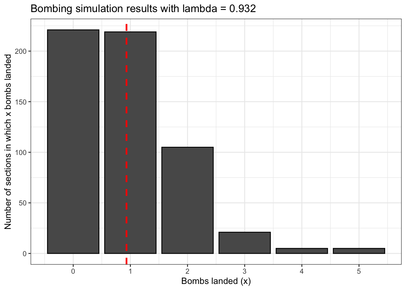
## 221 219 105  21   5   5
How do these simulated totals compared to what we would expect according to the Poisson distribution? Getting all of this data into a summary dataframe will be somewhat complicated, but the process is mostly familiar.
bombing_sim <- data.frame('sim_data' = bowls)

bombing_sim_summary <- data.frame('bombs_landed' = c('0', '1', '2', '3', '4', '5+'))

for (col in colnames(bombing_sim)){
  zero <- sum(bombing_sim[[col]] == 0)
  one <- sum(bombing_sim[[col]] == 1)
  two <- sum(bombing_sim[[col]] == 2)
  three <- sum(bombing_sim[[col]] == 3)
  four <- sum(bombing_sim[[col]] == 4)
  five_plus <- sum(bombing_sim[[col]] >= 5)

  column <- data.frame('simulated_total' = c(zero,
                                             one,
                                             two,
                                             three,
                                             four,
                                             five_plus))

  bombing_sim_summary <- cbind(bombing_sim_summary, column)
}

# calculation of theoretical totals
zero_to_four <- dpois(0:4, lambda) * u
five_plus <- ppois(4, lambda, lower.tail = FALSE) * u

theoretical_total <- data.frame('theoretical_total' = c(zero_to_four,
                                                        five_plus))


bombing_sim_summary <- cbind(bombing_sim_summary, round(theoretical_total, 2))

bombing_sim_summary
## bombs_landed simulated_total theoretical_total
## 1 0 221 226.74
## 2 1 219 211.39
## 3 2 105 98.54
## 4 3 21 30.62
## 5 4 5 7.14
## 6 5+ 5 1.57Notice how the theoretical probabilites were calculated. dpois() was used for the first five, but the last one required ppois(). Remember, when lower.tail = FALSE in a cumulative probability function in R, it calculates P(X > x). Here, it calculated P(X > 4) = P(X >= 5).
We’ll conclude with a visual summary of our bombing simulation results. The red dashed line is drawn at our value for lambda.
bombing_sim %>% ggplot() +
  geom_bar(aes(bowls),
           color = 'black') +
  geom_vline(xintercept = lambda,
             color = 'red',
             linetype = 'dashed',
             size = 1) +
  scale_x_continuous(breaks = 0:max(bowls)) +
  labs(x = 'Bombs landed (x)',
       y = 'Number of sections in which x bombs landed',
       title = 'Bombing simulation results with lambda = 0.932') +
  theme_bw()