2 The openair package
In this book two packages are frequently used and it is a good idea to load both.
Because the openair package (and R itself) are continually updated, it will be useful to know this document was produced using R version 4.4.0 and openair version 2.18.2.9004.
Where code is shown in this document, function names are hyper-linked and will take you to the help page for the function.
2.1 Installation and code access
openair is avaiable on CRAN (Comprehensive R Archive network) which means it can be installed easily from R. I would recommend re-starting R and then type install.packages("openair"). If you use RStudio (which is highly recommended), you can just choose the ‘packages’ tab on the bottom-right, and then select ‘Install’. Simply start typing openair and you will find the package.
For openair all development is carried out using Github for version control. Users can access all code used in openair at (https://github.com/davidcarslaw/openair).
Sometimes it might be useful to install the development version of openair and you can find instructions here.
2.2 Input data requirements
The openair package applies certain constraints on input data requirements. It is important to adhere to these requirements to ensure that data are correctly formatted for use in openair. The principal reason for insisting on specific input data format is that there will be less that can go wrong and it is easier to write code for a more limited set of conditions.
Data should be in a data frame (or
tibble).The date/time field should be called
date— note the lower case. No other name is acceptable.The wind speed and wind direction should be named
wsandwd, respectively (note again, lower case). Wind directions follow the UK Met Office format and are represented as degrees from north e.g. 90 degrees is east. North is taken to be 360 degreesWhere fields should have numeric data e.g. concentrations of NOx, then the user should ensure that no other characters are present in the column, accept maybe something that represents missing data e.g. ‘no data’.
Other variables names can be upper/lower case but should not start with a number. If column names do have white spaces, R will automatically replace them with a full-stop. While
PM2.5as a field name is perfectly acceptable, it is a pain to type it in—better just to usepm25(openair will recognise pollutant names like this and automatically format them as PM2.5 in plots).
2.3 Reading and formatting dates and times
While not specific to openair, dealing with dates and times is likely to be an issue that needs to be dealt with at some point. There is no getting away from the fact that dates and times can be complicated with issues such as time zones and daylight saving time i.e. when the clocks change for summer. This is a potentially big topic to consider and it is only considered in outline here.
For a lot of openair functions this issue will not be important. While these issues can often be ignored, it is better to be explicit and set the date-time correctly. Two situations where it becomes important is when wanting to show temporal variations in local time and combining data sets that are in different time zones. The former issue can be important (for example) when considering diurnal variations in a pollutant concentration that follows a human activity (such as rush-hour traffic), which follows local time and not GMT/UTC.
When importing data into R it is important to know how the date-time is represented in your original data, especially in terms of time zone.
When importing data it is important to know how the date-time is represented. In the UK it is easy for us to forget that simply working with data in GMT is not always an option. However, most air quality and meteorological data around the world tends to be in GMT/UTC or a fixed offset from GMT/UTC i.e. not in local time where hours can be missing or duplicated.
Life is made much easier using the lubridate package, which has been developed for working with dates and times. The lubridate package has a family of functions that will convert common formats of dates and times into a R-formatted version. These functions are useful when importing data and the date-time is in a character format and needs formatting. Here are some examples:
Original date in ‘British’ format (day/month/ year hours-minutes):
[1] "2022-08-02 11:00:00 UTC"When R formats a date-time correctly is will be shown from ‘large to small’ i.e. YYYY-MM-DD HH:MM:SS, which provides a clue that it has indeed been formatted correctly.
US date time with seconds (month-day-year):
date_time <- "8/2/2022 11:05:12"
mdy_hms(date_time)
[1] "2022-08-02 11:05:12 UTC"As you can see, by default, the date-time is formatted in UTC (GMT). It is at this point where you can also set a time zone of the original data if it was not in GMT. Let’s assume the original data were a fixed off-set from GMT of -8 hours (west coast USA perhaps). This can be done by setting the time zone explicitly1:
date_time <- "8/2/2022 11:05:12" # time 8 hours behind GMT
mdy_hms(date_time, tz = "Etc/GMT+8")
[1] "2022-08-02 11:05:12 -08"which actually shows the GMT offset of -8 hours.
A common task might be to plot time series and temporal variations of pollutant concentrations in local time. How does one do this if the imported data are in GMT/UTC (or a fixed offset from GMT/UTC)?
In this case it is necessary to know how the local time zone with daylight saving time (DST) is represented. Time zone names follow the Olson scheme — you can list them by typing OlsonNames(). Given the scenario where we have imported data in GMT but want to display the data in local time (BST — British Summer Time), we can use the with_tz function in lubridate to do this:
date_time <- "2/8/2022 11:00"

# format it
date_time <- dmy_hm(date_time) # GMT
date_time
[1] "2022-08-02 11:00:00 UTC"# what is the hour?
hour(date_time)[1] 11# format in local time
time_local <- with_tz(date_time, tz = "Europe/London")
time_local[1] "2022-08-02 12:00:00 BST"# local hour is +1 from GMT
hour(time_local)[1] 12In the above example, date_time and time_local are the same absolute time — we are just changing how the time is displayed. In practice, given a data frame with a date column in GMT and there interest in making sure openair uses the local time, some formatting such as mydata$date -> with_tz(mydata$date, tz = "Europe/London") is what is needed.
Another scenario is you import data using a function such as read_csv from the readr package and it recognises a date-time in the data and by default assumes it is GMT/UTC. This might be wrong even though it is now formatted correctly in R. In this case you can force a new time zone using the force_tz function. For example:
# a correctly formatted date-time that is in GMT but should be something else
date_time
[1] "2022-08-02 11:00:00 UTC"# force the time zone to be something different
force_tz(date_time, tz = "Etc/GMT+8")[1] "2022-08-02 11:00:00 -08"Finally, what about combining data sets in different time zones? In Chapter 4 it is shown how it is possible to access meteorological data from around the world (all in GMT). The interest might be in combining this data with air quality data that is in another time zone. So long as the date-times were correctly formatted in the first place, then simply joining the data sets by date is all that is needed, as R works out how the times match internally. An example of joining two data sets is shown in Section 4.2.
2.4 Brief overview of openair
This section gives a brief overview of the functions in openair. Having read some data into a data frame it is then straightforward to run any function. Almost all functions are run as:
functionName(thedata, options, ...)The usage is best illustrated through a specific example, in this case the polarPlot function. The details of the function are shown in Chapter 8 and through the help pages (type ?polarPlot). As it can be seen there are numerous options associated with polarPlot — and most other functions and each of these has a default. For example, the default pollutant considered in polarPlot is nox. If the user has a data frame called theData then polarPlot could minimally be called by:
polarPlot(theData)which would plot a nox polar plot if nox was available in the data frame theData.
Note that the options do not need to be specified in order nor is it always necessary to write the whole word. For example, it is possible to write:
polarPlot(theData, type = "year", poll = "so2")In this case writing poll is sufficient to uniquely identify that the option is pollutant.
Also there are many common options available in functions that are not explicitly documented, but are part of lattice graphics. Some common ones are summarised in Table 2.1. The layout option allows the user to control the layout of multi-panel plots e.g. layout = c(4, 1) would ensure a four-panel plot is 4 columns by 1 row.
| option | description |
|---|---|
| xlab | x-axis label |
| ylab | y-axis label |
| main | title of the plot |
| pch | plotting symbol used for points |
| cex | size of symbol plotted |
| lty | line type |
| lwd | line width |
| layout | the plot layout e.g. c(2, 2) |
2.5 The type option
One of the central themes in openair is the idea of conditioning. Rather than plot \(x\) against \(y\), considerably more information can usually be gained by considering a third variable, \(z\). In this case, \(x\) is plotted against \(y\) for many different intervals of \(z\). This idea can be further extended. For example, a trend of NOx against time can be conditioned in many ways: NOx vs. time split by wind sector, day of the week, wind speed, temperature, hour of the day … and so on. This type of analysis is rarely carried out when analysing air pollution data, in part because it is time consuming to do. However, thanks to the capabilities of R and packages such as lattice and ggplot2, it becomes easier to work in this way.
In most openair functions conditioning is controlled using the type option. type can be any other variable available in a data frame (numeric, character or factor). A simple example of type would be a variable representing a ‘before’ and ‘after’ situation, say a variable called period i.e. the option type = "period" is supplied. In this case a plot or analysis would be separately shown for ‘before’ and ‘after’. When type is a numeric variable then the data will be split into four quantiles and labelled accordingly. Note however the user can set the quantile intervals to other values using the option n.levels. For example, the user could choose to plot a variable by different levels of temperature. If n.levels = 3 then the data could be split by ‘low’, ‘medium’ and ‘high’ temperatures, and so on. Some variables are treated in a special way. For example if type = "wd" then the data are split into 8 wind sectors (N, NE, E, …) and plots are organised by points of the compass.
There are a series of pre-defined values that type can take related to the temporal components of the data as summarised in Table 2.2. To use these there must be a date field so that it can be calculated. These pre-defined values of type are shown below are both useful and convenient. Given a data frame containing several years of data it is easy to analyse the data e.g. plot it, by year by supplying the option type = "year". Other useful and straightforward values are “hour” and “month”. When type = "season" openair will split the data by the four seasons (winter = Dec/Jan/Feb etc.). Note for southern hemisphere users that the option hemisphere = "southern" can be given. When type = "daylight" is used the data are split between nighttime and daylight hours. In this case the user can also supply the options latitude and longitude for their location (the default is London).
type option that is available for most functions.
| option | description |
|---|---|
| ‘year’ | splits data by year |
| ‘month’ | splits data by month of the year |
| ‘week’ | splits data by week of the year |
| ‘monthyear’ | splits data by year and month |
| ‘season’ | splits data by season. Note in this case the user can also supply a hemisphere option that can be either ‘northern’ (default) or ‘southern’ |
| ‘weekday’ | splits data by day of the week |
| ‘weekend’ | splits data by Saturday, Sunday, weekday |
| ‘daylight’ | splits data by nighttime/daytime. Note the user must supply a longitude and latitude
|
| ‘dst’ | splits data by daylight saving time and non-daylight saving time |
| ‘wd’ | if wind direction (wd) is available type = 'wd' will split the data into 8 sectors: N, NE, E, SE, S, SW, W, NW |
| ‘seasonyear’ | will split the data into year-season intervals, keeping the months of a season together. For example, December 2010 is considered as part of winter 2011 (with January and February 2011). This makes it easier to consider contiguous seasons. In contrast, type = 'season' will just split the data into four seasons regardless of the year. |
If a categorical variable is present in a data frame e.g. site then that variables can be used directly e.g. type = "site".
2.5.1 Make your own type
In some cases it is useful to categorise numeric variables according to one’s own intervals. One example is air quality bands where concentrations might be described as “good”, “fair”, “bad”. For this situation we can use the cut function. In the example below, concentrations of NO2 are divided into intervals 0-50, 50-100, 100-150 and >150 using the breaks option. Also shown are user-defined labels. Note there is 1 more break than label. There are a couple of things to note here. First, include.lowest = TRUE ensures that the lowest value is included in the lowest break (in this case 0). Second, the maximum value (1000) is set to be more than the maximum value in the data to ensure the final break encompasses all the data.
mydata$intervals <- cut(mydata$no2,
                        breaks = c(0, 50, 100, 150, 1000),
                        labels = c("Very low", "Low", "High",
                                   "Very High"),
                        include.lowest = TRUE)

# look at the data
head(mydata)
# A tibble: 6 × 11
date ws wd nox no2 o3 pm10 so2 co pm25
<dttm> <dbl> <int> <int> <int> <int> <int> <dbl> <dbl> <int>
1 1998-01-01 00:00:00 0.6 280 285 39 1 29 4.72 3.37 NA
2 1998-01-01 01:00:00 2.16 230 NA NA NA 37 NA NA NA
3 1998-01-01 02:00:00 2.76 190 NA NA 3 34 6.83 9.60 NA
4 1998-01-01 03:00:00 2.16 170 493 52 3 35 7.66 10.2 NA
5 1998-01-01 04:00:00 2.4 180 468 78 2 34 8.07 8.91 NA
6 1998-01-01 05:00:00 3 190 264 42 0 16 5.50 3.05 NA
# ℹ 1 more variable: intervals <fct>Then it is possible to use the new intervals variable in most openair functions e.g. windRose(mydata, type = "intervals").
A special case is splitting data by date. In this scenario there might be interest in a ‘before-after’ situation e.g. due to an intervention. The openair function splitByDate should make this easy. Here is an example:
splitByDate(
  mydata,
  dates = "1/1/2003",
  labels = c("before", "after"),
  name = "scenario"
)
# A tibble: 65,533 × 12
date ws wd nox no2 o3 pm10 so2 co pm25
<dttm> <dbl> <int> <int> <int> <int> <int> <dbl> <dbl> <int>
1 1998-01-01 00:00:00 0.6 280 285 39 1 29 4.72 3.37 NA
2 1998-01-01 01:00:00 2.16 230 NA NA NA 37 NA NA NA
3 1998-01-01 02:00:00 2.76 190 NA NA 3 34 6.83 9.60 NA
4 1998-01-01 03:00:00 2.16 170 493 52 3 35 7.66 10.2 NA
5 1998-01-01 04:00:00 2.4 180 468 78 2 34 8.07 8.91 NA
6 1998-01-01 05:00:00 3 190 264 42 0 16 5.50 3.05 NA
7 1998-01-01 06:00:00 3 140 171 38 0 11 4.23 2.26 NA
8 1998-01-01 07:00:00 3 170 195 51 0 12 3.88 2.00 NA
9 1998-01-01 08:00:00 3.36 170 137 42 1 12 3.35 1.46 NA
10 1998-01-01 09:00:00 3.96 170 113 39 2 12 2.92 1.20 NA
# ℹ 65,523 more rows
# ℹ 2 more variables: intervals <fct>, scenario <ord>This code adds a new column scenario that is labelled before and after depending on the date. Note that the dates input by the user is in British format (dd/mm/YYYY) and that several dates (and labels) can be provided.
2.6 Controlling font size
All openair plot functions have an option fontsize. Users can easily vary the size of the font for each plot e.g.
polarPlot(mydata, fontsize = 20)The font size will be reset to the default sizes once the plot is complete. Finer control of individual font sizes is currently not easily possible.
2.7 Using colours
Many of the functions described require that colour scales are used; particularly for plots showing surfaces. It is only necessary to consider using other colours if the user does not wish to use the default scheme, shown at the top of Figure 2.1. The choice of colours does seem to be a vexing issue as well as something that depends on what one is trying to show in the first place. For this reason, the colour schemes used in openair are very flexible: if you don’t like them, you can change them easily. R itself can handle colours in many sophisticated ways; see for example the RColorBrewer package.
Several pre-defined colour schemes are available to make it easy to plot data. In fact, for most situations the default colour schemes should be adequate. The choice of colours can easily be set; either by using one of the pre-defined schemes or through a user-defined scheme. More details can be found in the openair openColours function. Some defined colours are shown in Figure 2.1, together with an example of a user defined scale that provides a smooth transition from red to green.
library(openair)
## small function for plotting
printCols <- function(col, y) {
  rect((0:200) / 200, y, (1:201) / 200, y + 0.1, col = openColours(col, n = 201),
       border = NA)
  text(0.5, y + 0.15, deparse(substitute(col)))
}

## plot an empty plot
plot(1, xlim = c(0, 1), ylim = c(0, 1.6), type = "n", xlab = "", ylab = "",
     axes = FALSE)
printCols("default", 0)
printCols("increment", 0.2)
printCols("heat", 0.4)
printCols("turbo", 0.6)
printCols("viridis", 0.8)
printCols("inferno", 1.0)
printCols("greyscale", 1.2)
printCols(c("tomato", "white", "forestgreen" ), 1.4)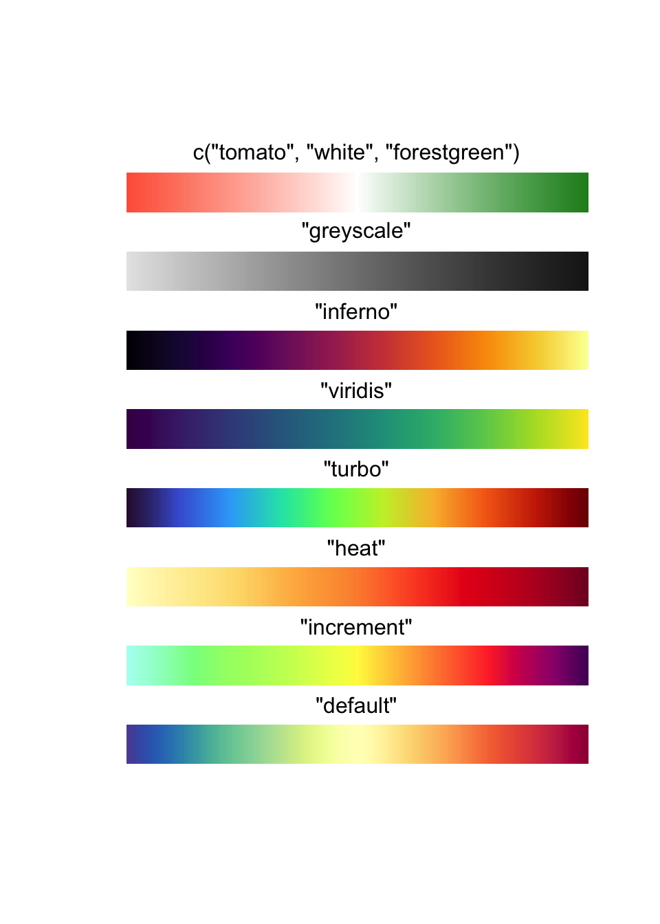
The user-defined scheme is very flexible and the following provides examples of its use. In the examples shown next, the polarPlot function is used as a demonstration of their use.
# use default colours - no need to specify
polarPlot(mydata)

# use pre-defined "turbo" colours
polarPlot(mydata, cols = "turbo")

# define own colours going from yellow to green
polarPlot(mydata, cols = c("yellow", "green"))

# define own colours going from red to white to blue
polarPlot(mydata, cols = c("red", "white", "blue"))
For more detailed information on using appropriate colours, have a look at the colorspace package. colorspace provides the definitive, comprehensive approach to using colours effectively. You will need to install the package, install.packages("colorspace"). To use the palettes with openair, you can for example do:
library(colorspace)
library(openair)
windRose(mydata, cols = qualitative_hcl(4, palette = "Dark 3"))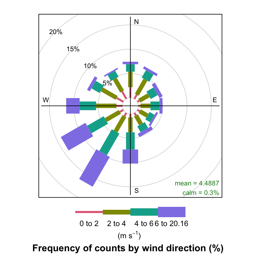
2.8 Automatic text formatting
openair tries to automate the process of annotating plots. It can be time-consuming (and tricky) to repetitively type in text to represent μg m-3 or PM10 (μg m-3) etc. in R. For this reason, an attempt is made to automatically detect strings such as nox or NOx and format them correctly. Where a user needs a y-axis label such as NOx (μg m-3) it will only be necessary to type ylab = "nox (ug/m3)". The same is also true for plot titles.
Users can override this option by setting it to FALSE.
2.9 Multiple plots on a page
We often get asked how to combine multiple plots on one page. Recent changes to openair makes this a bit easier. Note that because openair uses lattice graphics the base graphics par settings will not work.
It is possible to arrange plots based on a column \(\times\) row layout. Let’s put two plots side by side (2 columns, 1 row). First it is necessary to assign the plots to a variable:
Now we can plot them using the split option:
In the code above for the split option, the last two numbers give the overall layout (2, 1) — 2 columns, 1 row. The first two numbers give the column/row index for that particular plot. The last two numbers remain constant across the series of plots being plotted.
There is one difficulty with plots that already contain sub-plots such as timeVariation where it is necessary to identify the particular plot of interest (see the timeVariation help for details). However, say we want a polar plot (b above) and a diurnal plot:
c <- timeVariation(mydata)
print(b, split = c(1, 1, 2, 1))
print(c, split = c(2, 1, 2, 1), subset = "hour", newpage = FALSE)
For more control it is possible to use the position argument. position is a vector of 4 numbers, c(xmin, ymin, xmax, ymax) that give the lower-left and upper-right corners of a rectangle in which the plot is to be positioned. The coordinate system for this rectangle is [0–1] in both the x and y directions.
As an example, consider plotting the first plot in the lower left quadrant and the second plot in the upper right quadrant:
The position argument gives more fine control over the plot location.
2.10 Saving plots and data
While you’ll likely be using openair in an environment like RStudio, you’ll likely want to get the outputs of your analysis outside of RStudio to put into reports, papers, or other deliverables.
For data, this is relatively straightforward. The write.csv() function will write out a dataframe to a local file path. The only arguments it really needs is x (the dataframe to save) and file (the file path to save it to). For example, the below code chunk will load annual statistics for the Marylebone Road monitoring site, and save them to the path "my1_annual-stats_2022.csv". Always try to give files evocative names so you’ll know what’s in them in future - "my1_annual-stats_2022.csv" is better than "data.csv".
library(openair)

marylebone <-
  importUKAQ(site = "my1",
             year = 2022,
             source = "aurn",
             data_type = "annual",
             to_narrow = TRUE)

write.csv(x = marylebone, file = "my1_annual-stats_2022.csv")
Plots are slightly more complicated. If you do use RStudio, the simplest way to save an openair plot is to use the plots pane, visualised in Figure 2.3. This menu will allow you to copy your plot to the clipboard, or save it as an image or PDF.
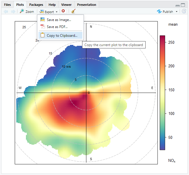
This may be useful in some scenarios, but using the RStudio GUI is not very reproducible. For sake of example, say you make a new set of plots every week for a weekly report. You may not want to have to repeatedly go into the plots pane, click ‘export’, set the correct dimensions, and so on every time a new plot needs to be saved. It would be preferable if your script created the plots and saved them!
To write a script to save a plot, use the following approach:
Create your openair plot, making sure to assign it (
<-) to a variable name.Open a graphics device, such as
png(),jpeg(),png(), and so on. This is the stage where you’ll set parameters like the width, height, and resolution. You’ll also need to define a path, much like when you save data. As before, give it an evocative name -"polarplot_marylebone_nox.png"is a lot more descriptive than"myplot.png". You’ll note that a file is created in your working directory, but it will be blank for the moment.Print the plot. In openair, this can typically achieved by simply printing the whole openair object. Note that the plot will not appear in your plots pane in RStudio - it is being printed to the file you’ve created.
Close the graphics device. This is simply achieved using
dev.off()regardless of your chosen device, and tells R to close the connection to the device. The image of the plot will now appear in the file you created in step 2.
Many R users will be familiar with ggplot2::ggsave() for saving plots. openair predates ggplot2, so this function will not work with openair plots.
You can read about R’s plotting devices by reading the “help” page for the png() function - type ?png into your console to bring it up.
The openairmaps package can create interactive HTML maps. To save these, you need to use the htmlwidgets::saveWidget() function. This is simpler than saving a static plot as you will not have to worry about resolution or dimensions.
library(openairmaps)

polarmap <- polarMap(polar_data, "nox")

htmlwidgets::saveWidget(widget = polarmap, file = "polarmap_london_nox.html")
Another way of sharing analysis produced using openair is in Quarto (or Rmarkdown) reports. These well documented on their respective websites.
As R help says: “Contrary to some expectations (but consistent with names such as ‘PST8PDT’), negative offsets are times ahead of (east of) UTC, positive offsets are times behind (west of) UTC.”↩︎