library(mgcv)
dat <- importUKAQ(site = "mh", year = 1988:2010)Appendix C — A closer look at trends
Understanding trends is a core component of air quality and the atmospheric sciences in general. openair provides two main functions for considering trends (smoothTrend and TheilSen; see Chapter 16 and Chapter 15, the latter useful for linear trend estimates. Understanding trends and quantifying them robustly is not so easy and careful analysis would treat each time series individually and consider a wide range of diagnostics. In this section we take advantage of some of the excellent capabilities that R has to consider fitting trend models. Experience with real atmospheric composition data shows that trends are rarely linear, which is unfortunate given how much of statistics has been built around the linear model.
Generalized Additive Models (GAMs) offer a flexible approach to calculating trends and in particular, the mgcv package contains many functions that are very useful for such modelling. Some of the details of this type of model are presented in Wood (2006) and the mgcv package itself.
Wood, S.N., 2006. Generalized additive models: An introduction with r. Chapman; Hall/CRC.
The example considered is 23 years of O3 measurements at Mace Head on the West coast of Ireland. The example shows the sorts of steps that might be taken to build a model to explain the trend. The data are first imported and then the year, month and trend estimated. Note that trend here is simply a decimal date that can be used to construct various explanatory models.
First we import the data:
## calculate monthly means
monthly <- timeAverage(dat, avg.time = "month")
## now calculate components for the models
monthly$year <- as.numeric(format(monthly$date, "%Y"))
monthly$month <- as.numeric(format(monthly$date, "%m"))
monthly <- transform(monthly, trend = year + (month - 1) / 12)
It is always a good idea to plot the data first:
timePlot(monthly, pollutant = "o3")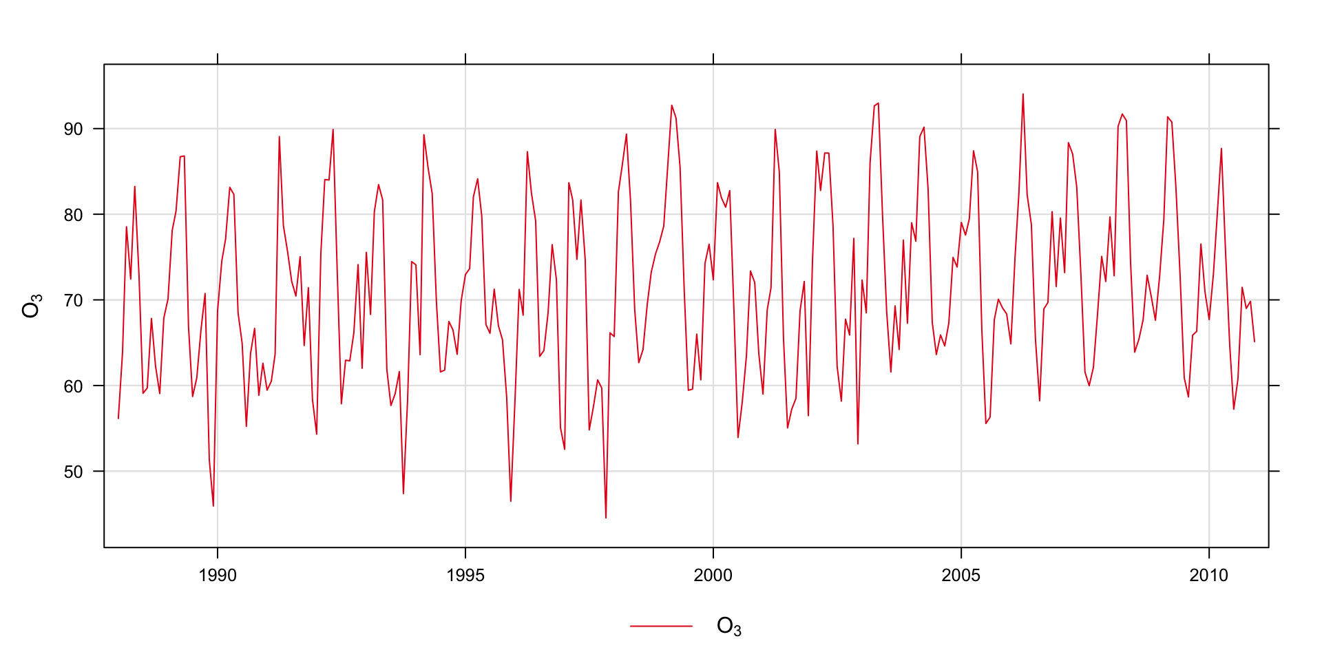
Figure C.1 shows that there is a clear seasonal variation in O3 concentrations, which is certainly expected. Less obvious is whether there is a trend.
Even though it is known there is a seasonal signal in the data, we will first of all ignore it and build a simple model that only has a trend component (model M0).
Family: gaussian
Link function: identity
Formula:
o3 ~ s(trend)
Parametric coefficients:
Estimate Std. Error t value Pr(>|t|)
(Intercept) 71.3428 0.6198 115.1 <2e-16 ***
---
Signif. codes: 0 '***' 0.001 '**' 0.01 '*' 0.05 '.' 0.1 ' ' 1
Approximate significance of smooth terms:
edf Ref.df F p-value
s(trend) 1 1 6.958 0.00882 **
---
Signif. codes: 0 '***' 0.001 '**' 0.01 '*' 0.05 '.' 0.1 ' ' 1
R-sq.(adj) = 0.0212 Deviance explained = 2.48%
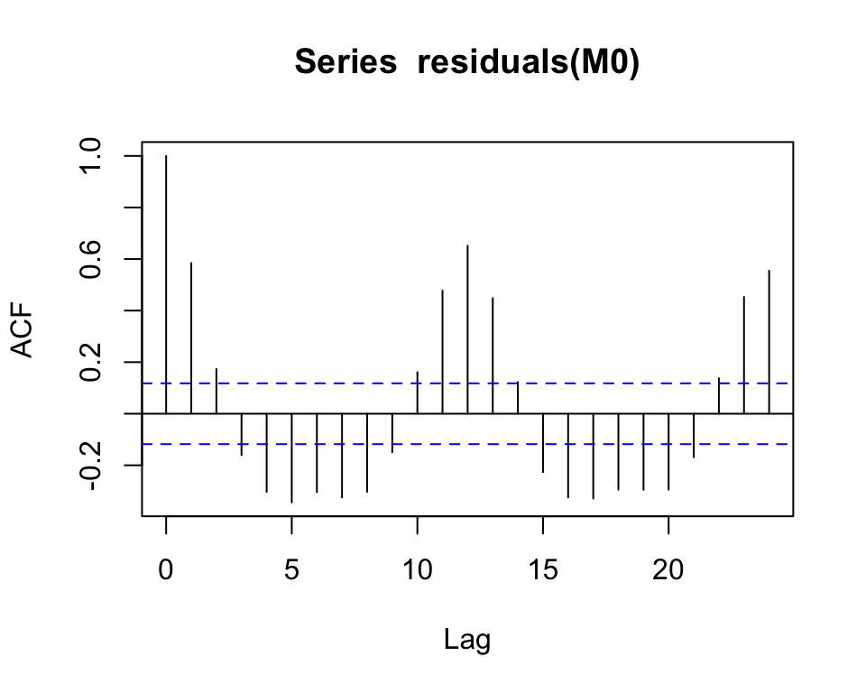
GCV = 106.82 Scale est. = 106.04 n = 276This model only explains about 2% of the variation as shown by the adjusted r2. More of a problem however is that no account has been taken of the seasonal variation. An easy way of seeing the effect of this omission is to plot the autocorrelation function (ACF) of the residuals, shown in Figure C.2. This Figure clearly shows the residuals have a strong seasonal pattern. Chatfield (2004) provides lots of useful information on time series modelling.
Chatfield, C., 2004. The analysis of time series : An introduction / chris chatfield, 6th ed. ed. Chapman & Hall/CRC, Boca Raton, FL ; London :
A refined model should therefore take account of the seasonal variation in O3 concentrations. Therefore, we add a term taking account of the seasonal variation. Note also that we choose a cyclic spline for the monthly component (bs = "cc"), which joins the first and last points i.e. January and December.
Family: gaussian
Link function: identity

Formula:
o3 ~ s(trend) + s(month, bs = "cc")

Parametric coefficients:
            Estimate Std. Error t value Pr(>|t|)
(Intercept)  71.3428     0.3738   190.9   <2e-16 ***
---
Signif. codes:  0 '***' 0.001 '**' 0.01 '*' 0.05 '.' 0.1 ' ' 1

Approximate significance of smooth terms:
           edf Ref.df     F  p-value
s(trend) 1.218  1.404 15.78 1.31e-05 ***
s(month) 6.111  8.000 59.35  < 2e-16 ***
---
Signif. codes:  0 '***' 0.001 '**' 0.01 '*' 0.05 '.' 0.1 ' ' 1

R-sq.(adj) =  0.644   Deviance explained = 65.4%
GCV = 39.766  Scale est. = 38.566    n = 276
Now we have a model that explains much more of the variation with an r2 of 0.65. Also, the p-values for the trend and seasonal components are both highly statistically significant. Let’s have a look at the separate components for trend and seasonal variation:
plot.gam(M1, select = 1, shade = TRUE)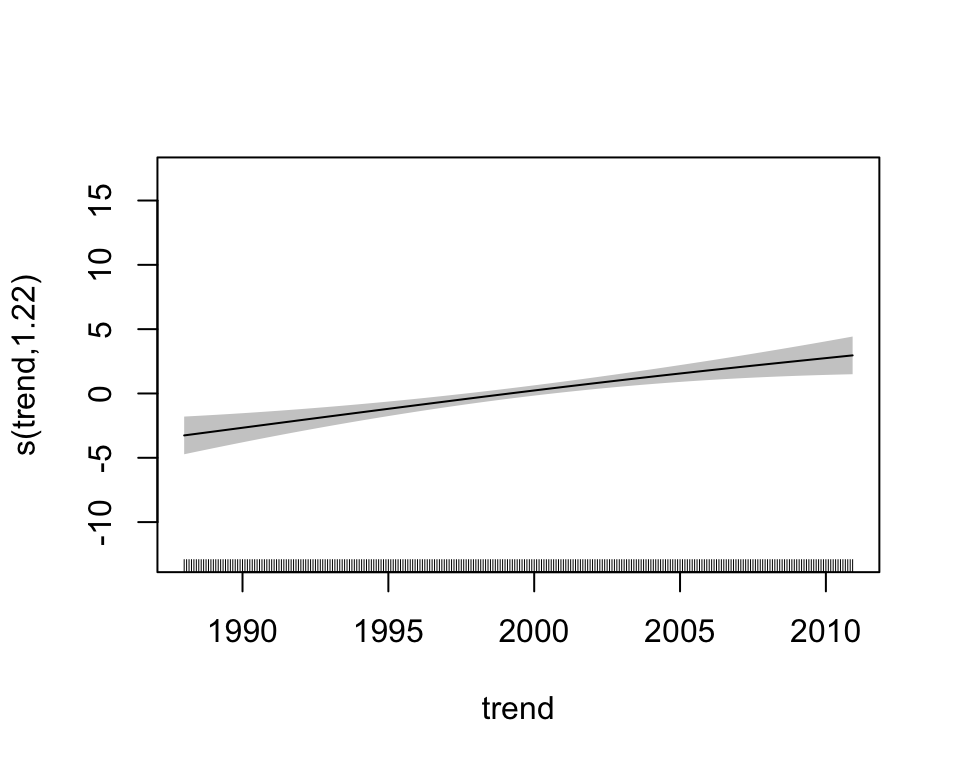
plot.gam(M1, select = 2, shade = TRUE)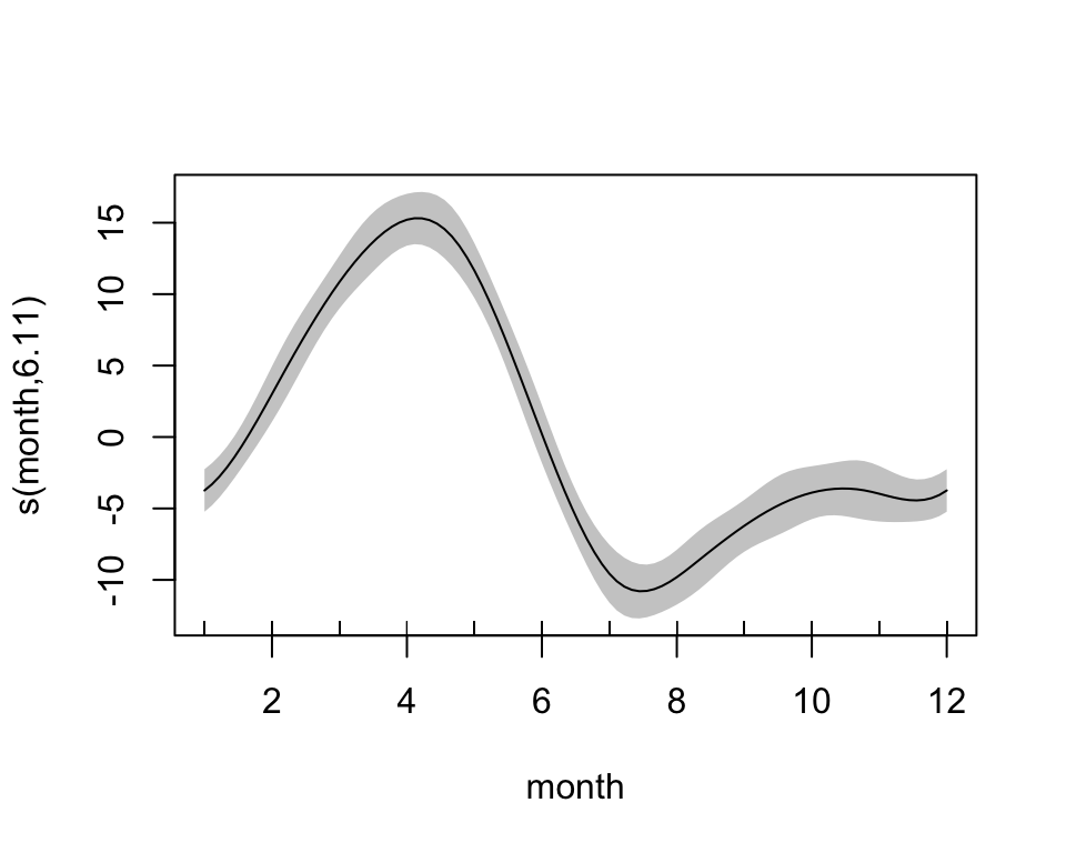
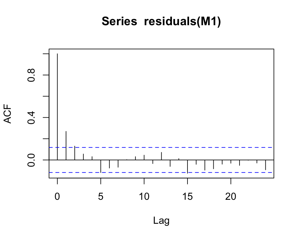
The seasonal component shown in Figure C.4 clearly shows the strong seasonal effect on O3 at this site (peaking in April). The trend component is actually linear in this case and could be modelled as such. This model looks much better, but as is often the case autocorrelation could remain important. The ACF is shown in Figure C.5 and shows there is still some short-term correlation in the residuals.
Note also that there are other diagnostic tests one should consider when comparing these models that are not shown here e.g. such as considering the normality of the residuals. Indeed a consideration of the residuals shows that the model fails to some extent in explaining the very low values of O3, which can be seen in Figure C.1. These few points (which skew the residuals) may well be associated with air masses from the polluted regions of Europe. Better and more useful models would likely be possible if the data were split by airmass origin, which is something that will be returned to when openair includes a consideration of back trajectories.
Further tests, also considering the partial autocorrelation function (PACF) suggest that an AR1 model is suitable for modelling this short-term autocorrelation. This is where modelling using a GAMM (Generalized Additive Mixed Model) comes in because it is possible to model the short-term autocorrelation using a linear mixed model. The gamm function uses the package nmle and the Generalized Linear Mixed Model (GLMM) fitting routine. In the M2 model below the correlation structure is considered explicitly.
M2 <- gamm(o3 ~ s(month, bs = "cc")  + s(trend),
           data = monthly,
           correlation = corAR1(form = ~ month | year))
summary(M2$gam)
Family: gaussian
Link function: identity
Formula:
o3 ~ s(month, bs = "cc") + s(trend)
Parametric coefficients:
Estimate Std. Error t value Pr(>|t|)
(Intercept) 71.3163 0.4933 144.6 <2e-16 ***
---
Signif. codes: 0 '***' 0.001 '**' 0.01 '*' 0.05 '.' 0.1 ' ' 1
Approximate significance of smooth terms:
edf Ref.df F p-value
s(month) 6.915 8 42.18 < 2e-16 ***
s(trend) 1.000 1 15.07 0.000131 ***
---
Signif. codes: 0 '***' 0.001 '**' 0.01 '*' 0.05 '.' 0.1 ' ' 1
R-sq.(adj) = 0.643
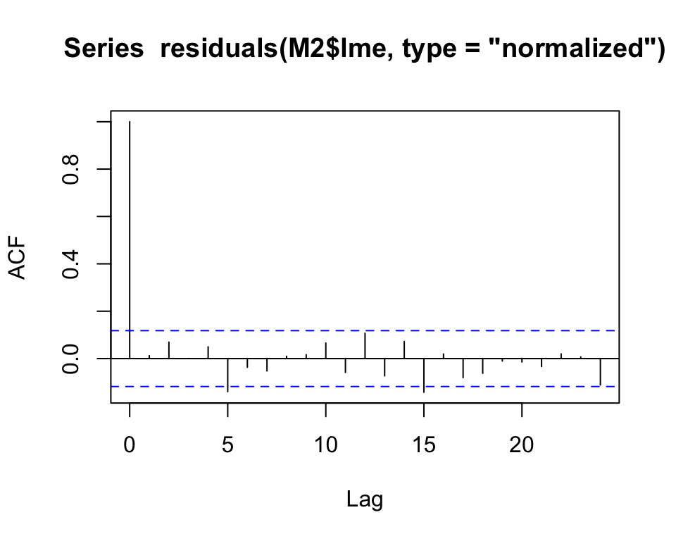
Scale est. = 38.863 n = 276The ACF plot is shown in Figure C.6 and shows that the autocorrelation has been dealt with and we can be rather more confident about the trend component (not plotted). Note that in this case we need to use the normalized residuals to get residuals that take account of the fitted correlation structure.
Note that model M2 assumes that the trend and seasonal terms vary independently of one another. However, if the seasonal amplitude and/or phase change over time then a model that accounts for the interaction between the two may be better. Indeed, this does seem to be the case here, as shown by the improved fit of the model below. This model uses a tensor product smooth (te) and the reason for doing this and not using an isotropic smooth (s) is that the trend and seasonal components are essentially on different scales. We would not necessarily want to apply the same level of smoothness to both components. An example of covariates on the same scale would be latitude and longitude.
M3 <- gamm(o3 ~ s(month, bs = "cc")  +
             te(trend, month), data = monthly,
           correlation = corAR1(form = ~ month | year))
summary(M3$gam)
Family: gaussian
Link function: identity

Formula:
o3 ~ s(month, bs = "cc") + te(trend, month)

Parametric coefficients:
            Estimate Std. Error t value Pr(>|t|)
(Intercept)  71.3213     0.4582   155.7   <2e-16 ***
---
Signif. codes:  0 '***' 0.001 '**' 0.01 '*' 0.05 '.' 0.1 ' ' 1

Approximate significance of smooth terms:
                  edf Ref.df      F  p-value
s(month)        6.886  8.000 22.205  < 2e-16 ***
te(trend,month) 4.163  4.163  7.961 8.04e-05 ***
---
Signif. codes:  0 '***' 0.001 '**' 0.01 '*' 0.05 '.' 0.1 ' ' 1

R-sq.(adj) =  0.667
  Scale est. = 36.121    n = 276
It becomes a bit more difficult to plot the two-way interaction between the trend and the month, but it is possible with a surface as shown in Figure C.7. This plot shows for example that during summertime the trends component varies little. However for the autumn and winter months there has been a much greater increase in the trend component for O3.
plot(M3$gam, select = 2, scheme = 1, theta = 225, phi = 10,ticktype = "detailed")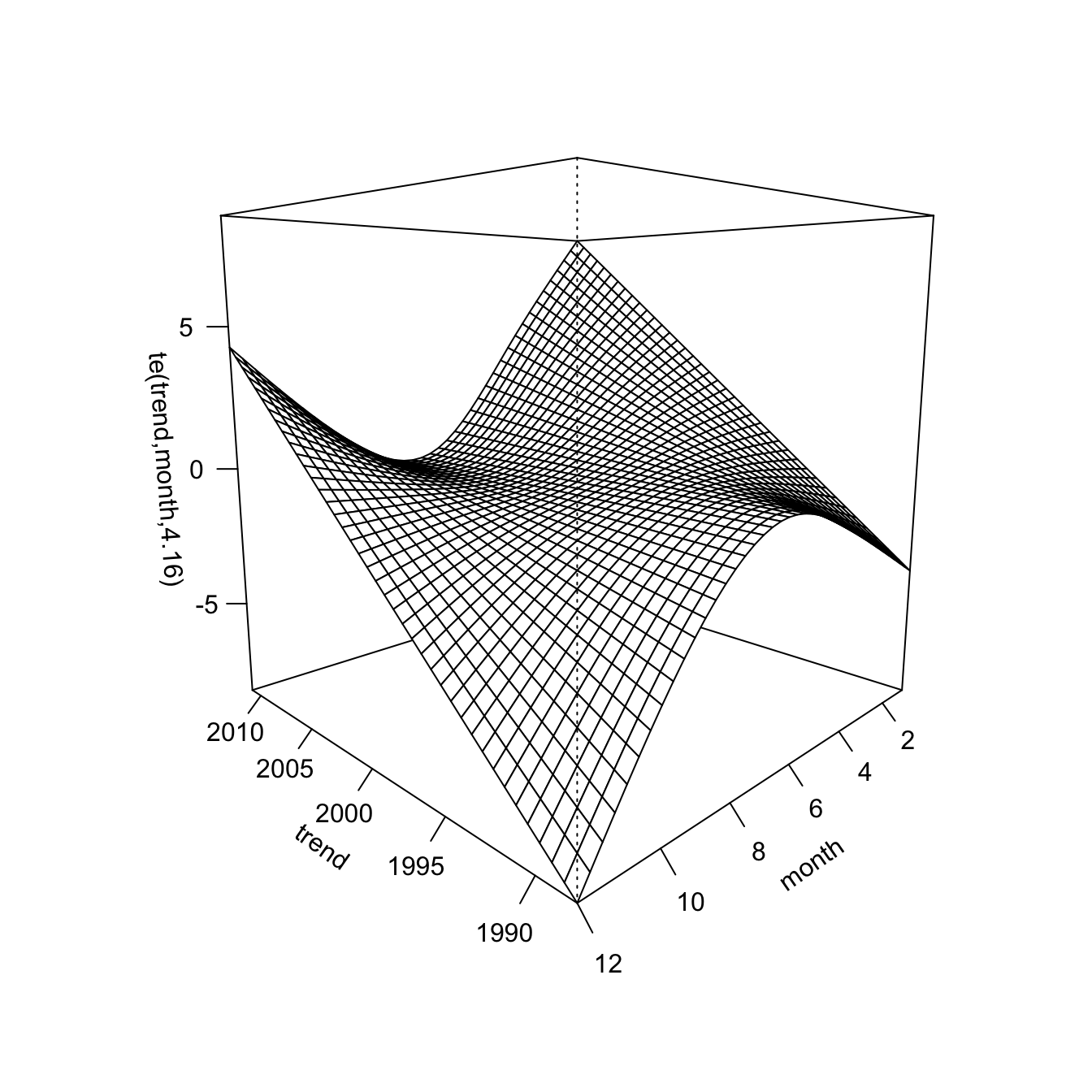
While there have been many steps involved in this short analysis, the data at Mace Head are not typical of most air quality data observed, say in urban areas. Much of the data considered in these areas does not appear to have significant autocorrelation in the residuals once the seasonal variation has been accounted for, therefore avoiding the complexities of taking account of the correlation structure of the data. It may be for example that sites like Mace Head and a pollutant such as O3 are much more prone to larger scale atmospheric processes that are not captured by these models.