percentileRose calculates percentile levels of a pollutant and plots them by wind direction. One or more percentile levels can be calculated and these are displayed as either filled areas or as lines.
By default, the function plots percentile concentrations in 10 degree segments. Alternatively, the levels by wind direction are calculated using a cyclic smooth cubic spline. The wind directions are rounded to the nearest 10 degrees, consistent with surface data from the UK Met Office before a smooth is fitted.
The percentileRose function complements other similar functions including windRose, pollutionRose, polarFreq or polarPlot. It is most useful for showing the distribution of concentrations by wind direction and often can reveal different sources e.g. those that only affect high percentile concentrations such as a chimney stack.
Similar to other functions, flexible conditioning is available through the type option. It is easy for example to consider multiple percentile values for a pollutant by season, year and so on. See examples below.
7.2 Examples
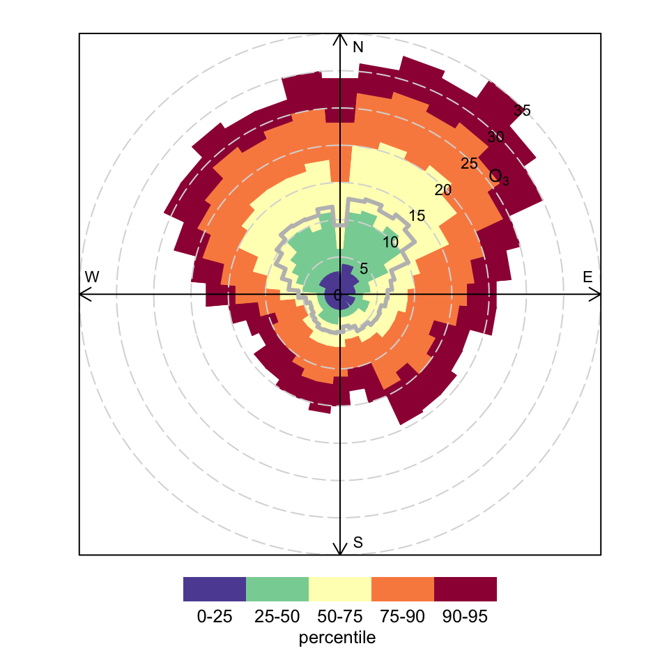
The first example is a basic plot of percentiles of O3 shown in Figure 7.1.
Figure 7.1: A percentileRose plot of O3 concentrations at Marylebone Road. The percentile intervals are shaded and are shown by wind direction. It shows for example that higher concentrations occur for northerly winds, as expected at this location. However, it also shows, for example the actual value of the 95th percentile O3 concentration.
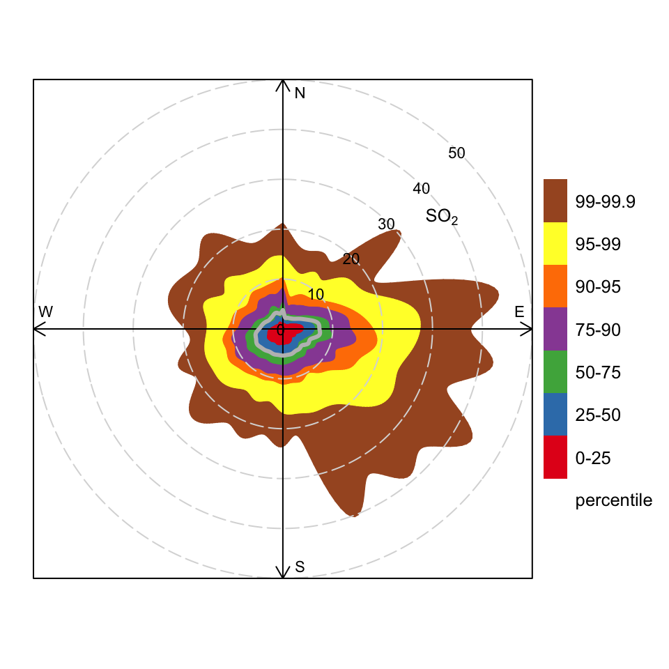
A slightly more interesting plot is shown in Figure 7.2 for SO2 concentrations. We also take the opportunity of changing some default options. In this case it can be clearly seen that the highest concentrations of SO2 are dominated by east and south-easterly winds; likely reflecting the influence of stack emissions in those directions.
Figure 7.2: A percentileRose plot of SO2 concentrations at Marylebone Road. The percentile intervals are shaded and are shown by wind direction. This plot sets some user-defined percentile levels to consider the higher SO2 concentrations, moves the key to the right and uses an alternative colour scheme.
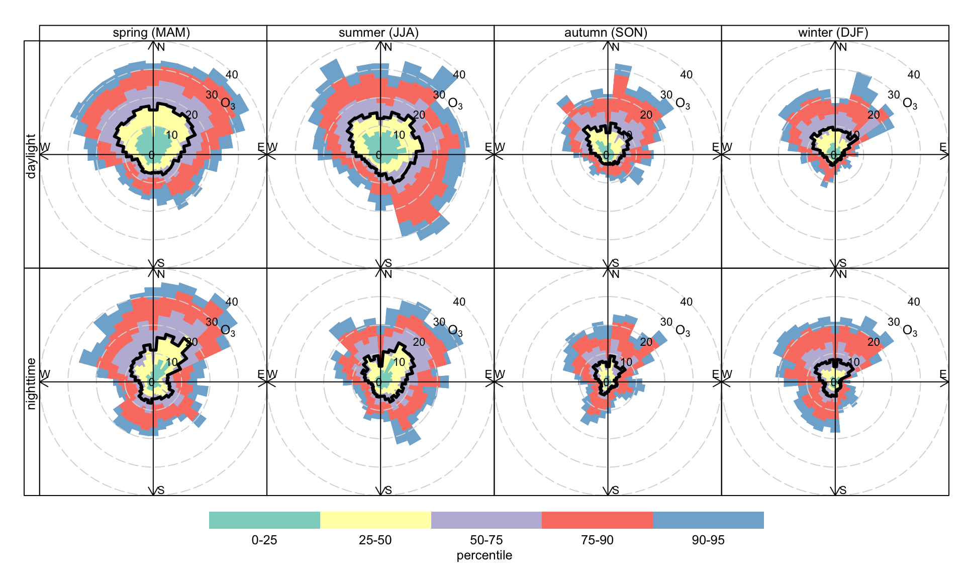
Lots more insight can be gained by considering how percentile values vary by other factors i.e. conditioning. For example, what do O3 concentrations look like split by season and whether it is daylight or nighttime hours? We can set the type to consider season and whether it is daylight or nighttime.1 This Figure reveals some interesting features. First, O3 concentrations are higher in the spring and summer and when the wind is from the north. O3 concentrations are higher on average at this site in spring due to the peak of northern hemispheric O3 and to some extent local production. This may also explain why O3 concentrations are somewhat higher at nighttime in spring compared with summer. Second, peak O3 concentrations are higher during daylight hours in summer when the wind is from the south-east. This will be due to more local (UK/European) production that is photochemically driven — and hence more important during daylight hours.
percentileRose(mydata, type =c("season", "daylight"), pollutant ="o3", col ="Set3", mean.col ="black")
Figure 7.3: A percentileRose plot of O3 concentrations at Marylebone Road. The percentile intervals are shaded and are shown by wind direction.The plot shows the variation by season and whether it is nighttime or daylight hours.
7.3 Condtional probability function
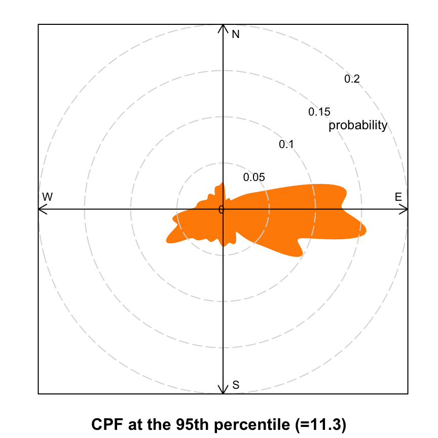
The percentileRose function can also plot conditional probability functions (CPF) (Ashbaugh et al., 1985). The CPF is defined as CPF = \(m_\theta/n_\theta\), where \(m_\theta\) is the number of samples in the wind sector \(\theta\) with mixing ratios greater than some high concentration, and \(n_\theta\) is the total number of samples in the same wind sector. CPF analysis is very useful for showing which wind directions are dominated by high concentrations and give the probability of doing so. In openair, a CPF plot can be produced as shown in Figure 7.4. Note that in these plots only one percentile is provided and the method must be supplied. In Figure 7.4 it is clear that the high concentrations (greater than the 95th percentile of all observations) is dominated by easterly wind directions. There are very low conditional probabilities of these concentrations being experienced for other wind directions.
Ashbaugh, L.L., Malm, W.C., Sadeh, W.Z., 1985. A residence time probability analysis of sulfur concentrations at grand Canyon National Park. Atmospheric Environment (1967) 19, 1263–1270. https://doi.org/10.1016/0004-6981(85)90256-2
percentileRose(mydata, poll="so2", percentile =95, method ="cpf", col ="darkorange", smooth =TRUE)
Figure 7.4: A CPF plot of SO2 concentrations at Marylebone Road.
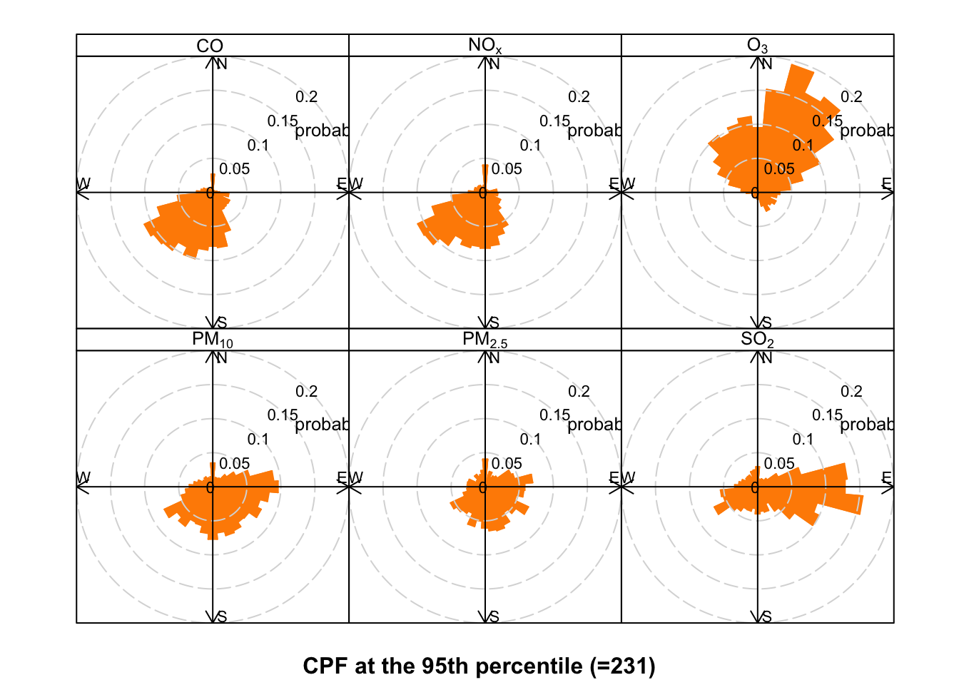
It is easy to plot several species on the same plot and this works well because they all have the same probability scale (i.e. 0 to 1). In the example below Figure 7.5 it is easy to see for each pollutant the wind directions that dominate the contributions to the highest (95th percentile) concentrations. For example, the highest CO and NOx concentrations are totally dominated by south/south-westerly winds and the probability of their being such high concentrations from other wind directions is effectively zero.
Figure 7.5: A CPF plot of many pollutants at Marylebone Road.
In choosing type = "daylight" the default is to consider a latitude of central London (or close to). Users can set the latitude in the function call if working in other parts of the world.↩︎