10 Trajectory analysis
10.1 Introduction
Back trajectories are extremely useful in air pollution and can provide important information on air mass origins. Despite the clear usefulness of back trajectories, their use tends to be restricted to the research community. Back trajectories are used for many purposes from understanding the origins of air masses over a few days to undertaking longer term analyses. They are often used to filter air mass origins to allow for more refined analyses of air pollution — for example trends in concentration by air mass origin. They are often also combined with more sophisticated analyses such as cluster analysis to help group similar type of air mass by origin.
Perhaps one of the reasons why back trajectory analysis is not carried out more often is that it can be time consuming to do. This is particularly so if one wants to consider several years at several sites. It can also be difficult to access back trajectory data. In an attempt to overcome some of these issues and expand the possibilities for data analysis, openair makes several functions available to access and analyse pre-calculated back trajectories.
Currently these functions allow for the import of pre-calculated back trajectories are several pre-define locations and some trajectory plotting functions. In time all of these functions will be developed to allow more sophisticated analyses to be undertaken. .
The importTraj() function imports pre-calculated back trajectories using the Hysplit trajectory model Hybrid Single Particle Lagrangian Integrated Trajectory Model (Stein et al., 2015). Trajectories are run at 3-hour intervals and stored in yearly files (see below). The trajectories are started at ground-level (10m) and propagated backwards in time. The data are stored on web-servers at Ricardo Energy & Environment similar to that for importUKAQ, which makes it very easy to import pre-processed trajectory data for a range of locations and years. 1
Users may for various reasons wish to run Hysplit themselves e.g. for different starting heights, longer periods or more locations. Code and instructions have been provided in Appendix B for users wishing to do this. Users can also use different means of calculating back trajectories e.g. ECMWF and plot them in openair provided a few basic fields are present: date (POSIXct), lat (decimal latitude), lon (decimal longitude) and hour.inc the hour offset from the arrival date (i.e. from zero decreasing to the length of the back trajectories). See ?importTraj for more details.
These trajectories have been calculated using the Global NOAA-NCEP/NCAR reanalysis data archives. The global data are on a latitude-longitude grid (2.5°). Note that there are many meteorological data sets that can be used to run Hysplit e.g. including ECMWF data. However, in order to make it practicable to run and store trajectories for many years and sites, the NOAA-NCEP/NCAR reanalysis data is most useful. In addition, these archives are available for use widely, which is not the case for many other data sets e.g. ECMWF. Hysplit calculated trajectories based on archive data may be distributed without permission (see https://ready.arl.noaa.gov/HYSPLIT_agreement.php). For those wanting, for example, to consider higher resolution meteorological data sets it may be better to run the trajectories separately.
openair uses the mapproj package to allow users to user different map projections. By default, the projection used is Lambert conformal, which is a conic projection best used for mid-latitude areas. The Hysplit model itself will use any one of three different projections depending on the latitude of the origin. If the latitude greater than 55.0 (or less than -55.0) then a polar stereographic projection is used, if the latitude greater than -25.0 and less than 25.0 the mercator projection is used and elsewhere (the mid-latitudes) the Lambert projection. All these projections (and many others) are available in the mapproj package.
Users should see the help file for importTraj to get an up to date list of receptors where back trajectories have been calculated. First, the packages are loaded that are needed.
As an example, we will import trajectories for London in 2010. Importing them is easy:
traj <- importTraj(site = "london", year = 2010)The file itself contains lots of information that is of use for plotting back trajectories:
head(traj) receptor year month day hour hour.inc lat lon height pressure
1 1 2010 1 1 9 0 51.500 -0.100 10.0 994.7
2 1 2010 1 1 8 -1 51.766 0.057 10.3 994.9
3 1 2010 1 1 7 -2 52.030 0.250 10.5 995.0
4 1 2010 1 1 6 -3 52.295 0.488 10.8 995.0
5 1 2010 1 1 5 -4 52.554 0.767 11.0 995.4
6 1 2010 1 1 4 -5 52.797 1.065 11.3 995.6
date2 date
1 2010-01-01 09:00:00 2010-01-01 09:00:00
2 2010-01-01 08:00:00 2010-01-01 09:00:00
3 2010-01-01 07:00:00 2010-01-01 09:00:00
4 2010-01-01 06:00:00 2010-01-01 09:00:00
5 2010-01-01 05:00:00 2010-01-01 09:00:00
6 2010-01-01 04:00:00 2010-01-01 09:00:00The traj data frame contains among other things the latitude and longitude of the back trajectory, the height (m) and pressure (Pa) of the trajectory. The date field is the arrival time of the air-mass and is useful for linking with ambient measurement data.
The trajPlot function is used for plotting back trajectory lines and density plots and has the following options:
10.2 Plotting trajectories
Next, we consider how to plot back trajectories with a few simple examples. The first example will consider a potentially interesting period when the Icelandic volcano, Eyjafjallajokull erupted in April 2010. The eruption of Eyjafjallajokull resulted in a flight-ban that lasted six days across many European airports. In Figure 10.1 selectByDate is used to consider the 7 days of interest and we choose to plot the back trajectories as lines rather than points (the default). Figure 10.1 does indeed show that many of the back trajectories originated from Iceland over this period. Note also the plot automatically includes a world base map. The base map itself is not at very high resolution by default but is useful for the sorts of spatial scales that back trajectories exist over. The base map is also global, so provided that there are pre-calculated back trajectories, these maps can be generated anywhere in the world. By default the function uses the ‘world’ map from the maps package. If map.res = "hires" then the (much) more detailed base map worldHires from the mapdata package is used.2
selectByDate(traj,
  start = "15/4/2010",
  end = "21/4/2010"
) %>%
  trajPlot(
    map.cols = openColours("hue", 10),
    col = "grey30"
  )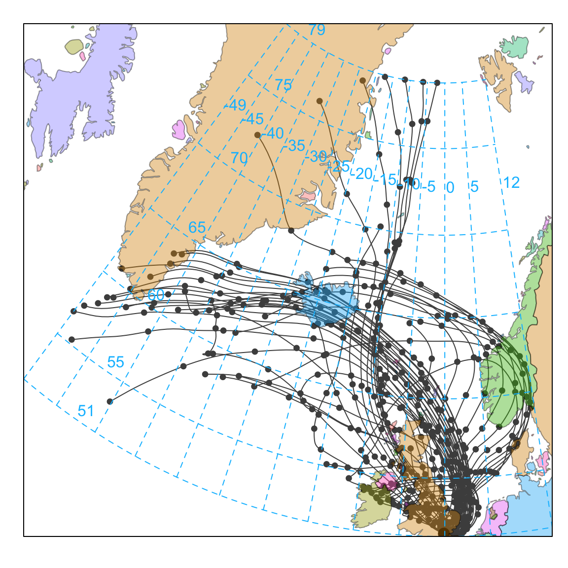
map.cols. By default the map colours for all countries are grey.
Note that trajPlot will only plot full length trajectories. This can be important when plotting something like a single month e.g. by using selectByDate when on partial sections of some trajectories may be selected.
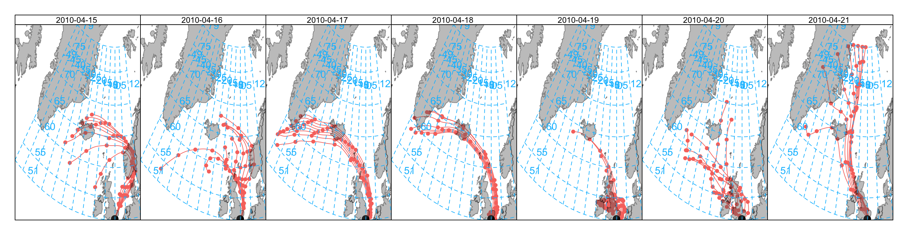
There are a few other ways of representing the data shown in Figure 10.1. For example, it might be useful to plot the trajectories for each day. To do this we need to make a new column day which can be used in the plotting. The first example considers plotting the back trajectories in separate panels (Figure 10.2).
## make a day column
traj$day <- as.Date(traj$date)

## plot it choosing a specific layout
selectByDate(traj,
  start = "15/4/2010",
  end = "21/4/2010"
) %>%
  trajPlot(
    type = "day",
    layout = c(7, 1)
  )
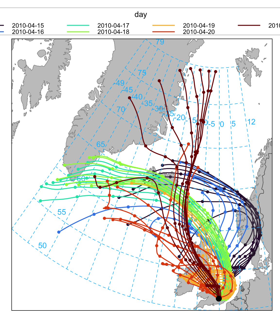
Another way of plotting the data is to group the trajectories by day and colour them. This time we also set a few other options to get the layout we want — shown in Figure 10.3.
selectByDate(traj,
  start = "15/4/2010",
  end = "21/4/2010"
) %>%
  trajPlot(
    group = "day", col = "turbo",
    lwd = 2, key.pos = "top",
    key.col = 4,
    ylim = c(50, 79)
  )
So far the plots have provided information on where the back trajectories come from, grouped or split by day. It is also possible, in common with most other openair functions to split the trajectories by many other variables e.g. month, season and so on. However, perhaps one of the most useful approaches is to link the back trajectories with the concentrations of a pollutant. As mentioned previously, the back trajectory data has a column date representing the arrival time of the air mass that can be used to link with concentration measurements. A couple of steps are required to do this using the left_join function.
## import data for North Kensington
kc1 <- importUKAQ("kc1", year = 2010)
# now merge with trajectory data by 'date'
traj <- left_join(traj, kc1, by = "date")
## look at first few lines
head(traj)
receptor year month day hour hour.inc lat lon height pressure
1 1 2010 1 2010-01-01 9 0 51.500 -0.100 10.0 994.7
2 1 2010 1 2010-01-01 8 -1 51.766 0.057 10.3 994.9
3 1 2010 1 2010-01-01 7 -2 52.030 0.250 10.5 995.0
4 1 2010 1 2010-01-01 6 -3 52.295 0.488 10.8 995.0
5 1 2010 1 2010-01-01 5 -4 52.554 0.767 11.0 995.4
6 1 2010 1 2010-01-01 4 -5 52.797 1.065 11.3 995.6
date2 date source site code co
1 2010-01-01 09:00:00 2010-01-01 09:00:00 aurn London N. Kensington KC1 0.3
2 2010-01-01 08:00:00 2010-01-01 09:00:00 aurn London N. Kensington KC1 0.3
3 2010-01-01 07:00:00 2010-01-01 09:00:00 aurn London N. Kensington KC1 0.3
4 2010-01-01 06:00:00 2010-01-01 09:00:00 aurn London N. Kensington KC1 0.3
5 2010-01-01 05:00:00 2010-01-01 09:00:00 aurn London N. Kensington KC1 0.3
6 2010-01-01 04:00:00 2010-01-01 09:00:00 aurn London N. Kensington KC1 0.3
nox no2 no o3 so2 pm10 pm2.5 v10 v2.5 nv10 nv2.5 ws wd air_temp
1 38 29 6 46 0 8 NA 0 NA 8 NA NA NA NA
2 38 29 6 46 0 8 NA 0 NA 8 NA NA NA NA
3 38 29 6 46 0 8 NA 0 NA 8 NA NA NA NA
4 38 29 6 46 0 8 NA 0 NA 8 NA NA NA NA
5 38 29 6 46 0 8 NA 0 NA 8 NA NA NA NA
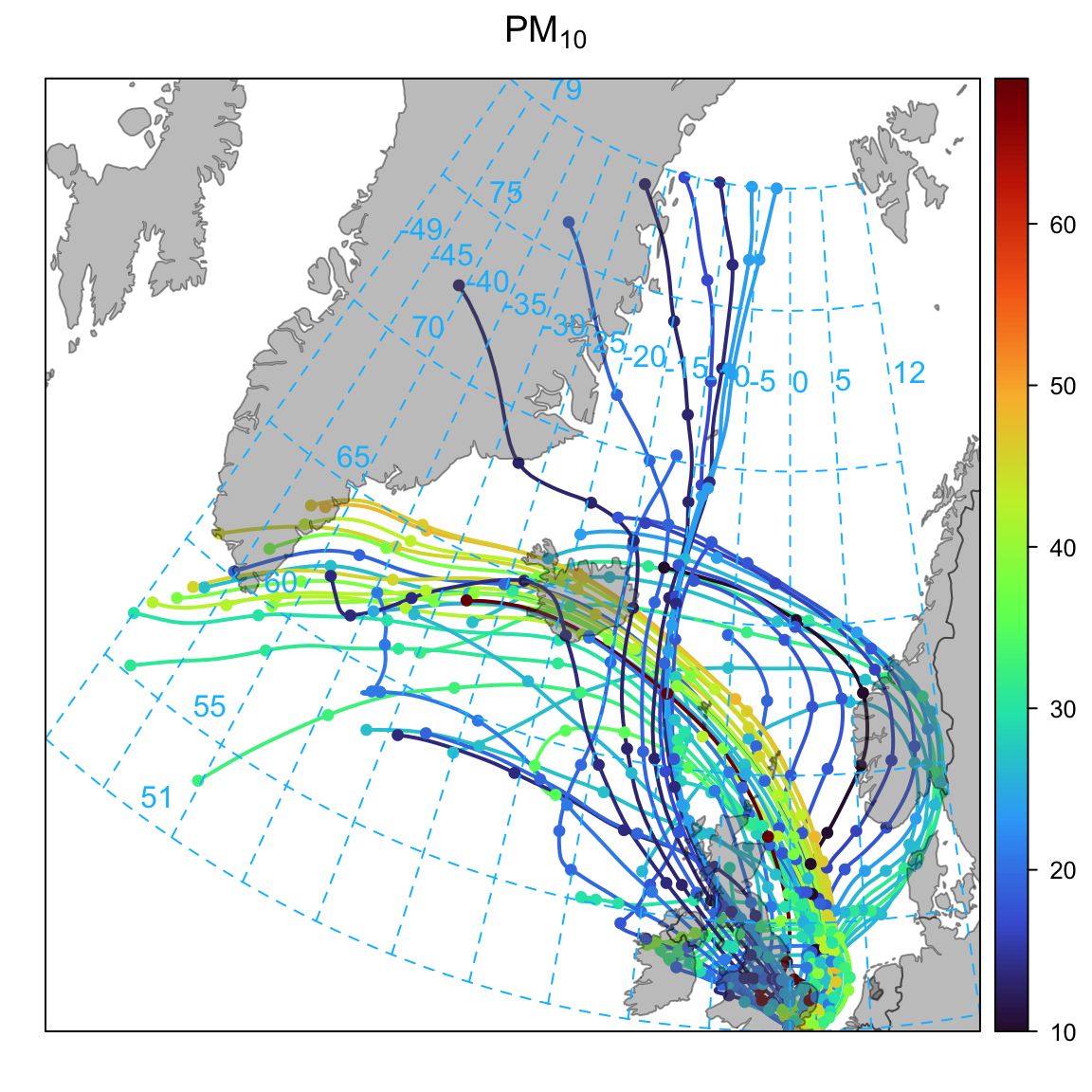
6 38 29 6 46 0 8 NA 0 NA 8 NA NA NA NAThis time we can use the option pollutant in the function trajPlot, which will plot the back trajectories coloured by the concentration of a pollutant. Figure 10.4 does seem to show elevated PM10 concentrations originating from Iceland over the period of interest. In fact, these elevated concentrations occur on two days as shown in Figure 10.2. However, care is needed when interpreting such data because other analysis would need to rule out other reasons why PM10 could be elevated; in particular due to local sources of PM10. There are lots of openair functions that can help here e.g. timeVariation or timePlot to see if NOx concentrations were also elevated (which they seem to be). It would also be worth considering other sites for back trajectories that could be less influenced by local emissions.
selectByDate(traj,
  start = "15/4/2010",
  end = "21/4/2010"
) %>%
  trajPlot(
    pollutant = "pm10",
    col = "turbo", lwd = 2
  )
However, it is possible to account for the PM that is local to some extent by considering the relationship between NOx and PM10 (or PM2.5). For example, using scatterPlot (not shown):
scatterPlot(kc1, x = "nox",
            y = "pm2.5",
            avg = "day",
            linear = TRUE)
which suggests a gradient of 0.084. Therefore, we can remove the PM10 that is associated NOx in kc1 data, making a new column pm.new:
kc1 <- mutate(kc1, pm.new = pm10 - 0.084 * nox)We have already merged kc1 with traj, so to keep things simple we import traj again and merge it with kc1. Note that if we had thought of this initially, pm.new would have been calculated first before merging with traj.
traj <- importTraj(site = "london", year = 2010)
traj <- left_join(traj, kc1, by = "date")
Now it is possible to plot the trajectories:
selectByDate(traj,
  start = "15/4/2010",
  end = "21/4/2010"
) %>%
  trajPlot(
    pollutant = "pm.new",
    col = "turbo", lwd = 2
  )
Which, interestingly still clearly shows elevated PM10 concentrations for those two days that cross Iceland. The same is also true for PM2.5. However, as mentioned previously, checking other sites in more rural areas would be a good idea.
10.3 Trajectory gridded frequencies
The Hysplit model itself contains various analysis options for gridding trajectory data. Similar capabilities are also available in openair where the analyses can be extended using other openair capabilities. It is useful to gain an idea of where trajectories come from. Over the course of a year representing trajectories as lines or points results in a lot of over-plotting. Therefore it is useful to grid the trajectory data and calculate various statistics by considering latitude-longitude intervals. The first analysis considers the number of unique trajectories in a particular grid square. This is achieved by using the trajLevel function and setting the statistic option to “frequency”. Figure 10.5 shows the frequency of back trajectory crossings for the London data. In this case it highlights that most trajectory origins are from the west and north for 2010 at this site. Note that in this case, pollutant can just be the trajectory height (or another numeric field) rather than an actual pollutant because only the frequencies are considered.
trajLevel(traj, statistic = "frequency")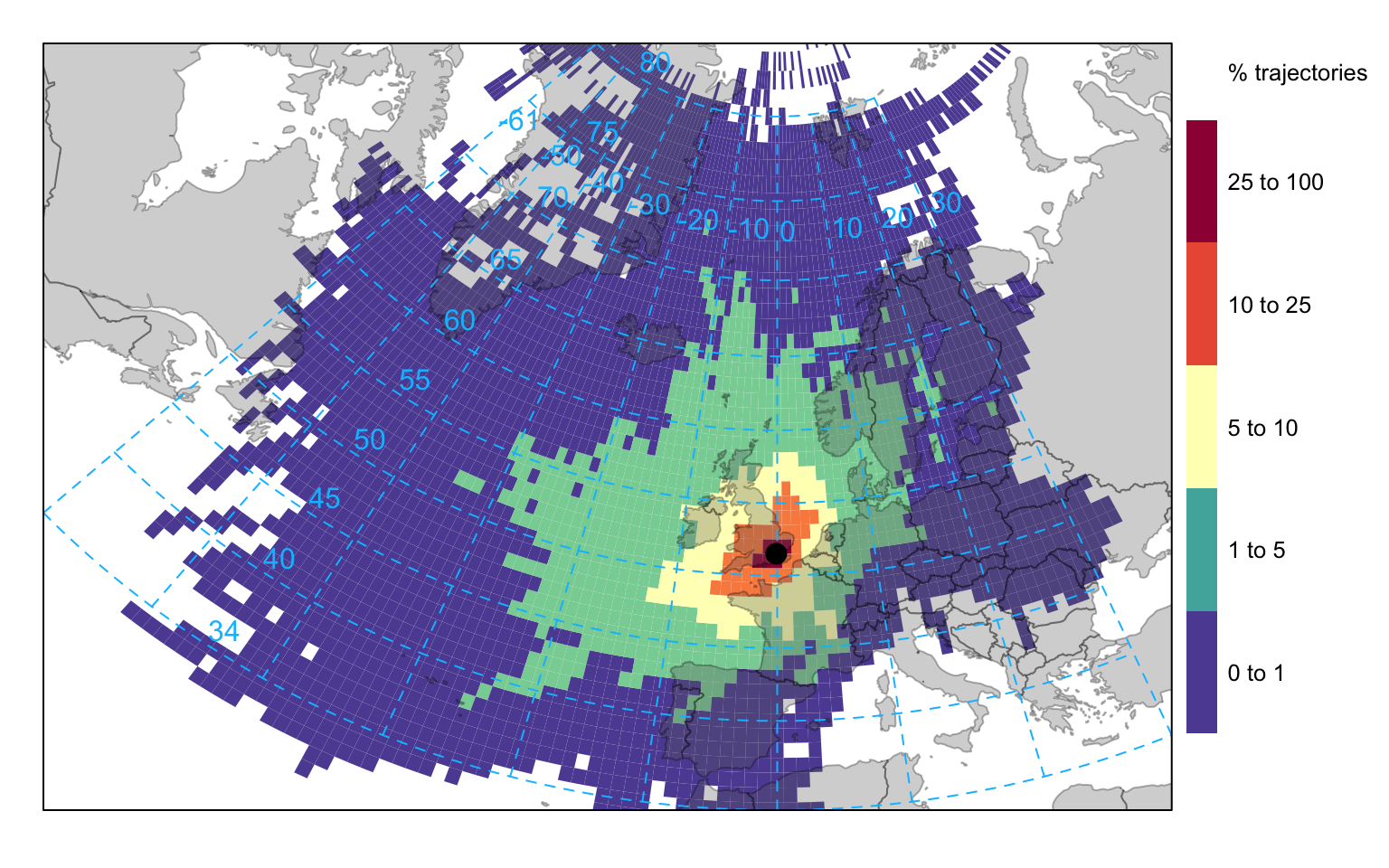
border = NA option removes the border around each grid cell.
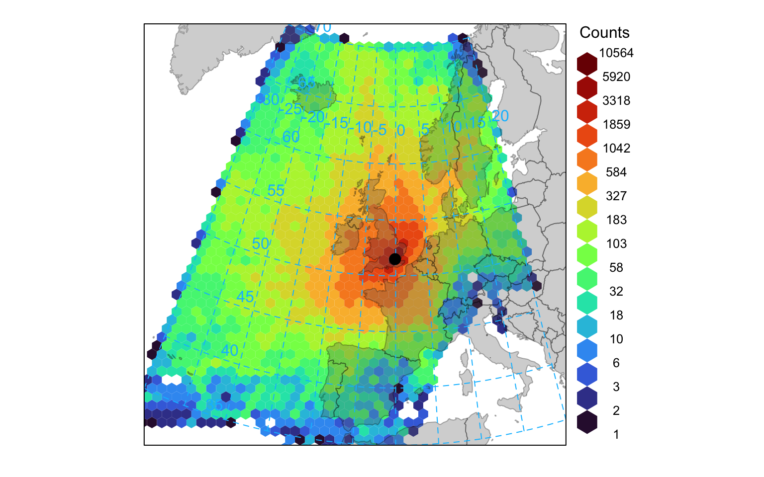
It is also possible to use hexagonal binning to gain an idea about trajectory frequencies. In this case each 3-hour point along each trajectory is used in the counting. The code below focuses more on Europe and uses the hexagonal binning method. Note that the effect of the very few high number of points at the origin has been diminished by plotting the data on a log scale — see Section 27.2.1 for details.
10.4 Trajectory source contribution functions
Back trajectories offer the possibility to undertake receptor modelling to identify the location of major emission sources. When many back trajectories (over months to years) are analysed in specific ways they begin to show the geographic origin most associated with elevated concentrations. With enough (dissimilar) trajectories those locations leading to the highest concentrations begin to be revealed. When a whole year of back trajectory data is plotted the individual back trajectories can extend 1000s of km. There are many approaches using back trajectories in this way and (Fleming et al., 2012) provide a good overview of the methods available. openair has implemented a few of these techniques and over time these will be refined and extended.
10.4.1 Identifying the contribution of high concentration back trajectories
A useful analysis to undertake is to consider the pattern of frequencies for two different conditions. In particular, there is often interest in the origin of high concentrations for different pollutants. For example, compared with data over a whole year, how do the frequencies of occurrence differ? Figure 10.7 shows an example of such an analysis for PM10 concentrations. By default the function will compare concentrations >90th percentile with the full year. The percentile level is controlled by the option percentile. Note also there is an option min.bin that will exclude grid cells where there are fewer than min.bin data points. The analysis compares the percentage of time the air masses are in particular grid squares for all data and a subset of data where the concentrations are greater than the given percentile. The graph shows the absolute percentage difference between the two cases i.e. high minus base.
Figure 10.7 shows that compared with the whole year, high PM10 concentrations (90th percentile) are more prevalent when the trajectories originate from the east, which is seen by the positive values in the plot. Similarly there are relatively fewer occurrences of these high concentration back trajectories when they originate from the west. This analysis is in keeping with the highest PM10 concentrations being largely controlled by secondary aerosol formation from air-masses originating during anticyclonic conditions from mainland Europe.
trajLevel(traj, pollutant = "pm10",
          statistic = "difference",
          col = c("skyblue", "white", "tomato"),
          min.bin = 50,
          border = NA,
          xlim = c(-20, 20),
          ylim = c(40, 70))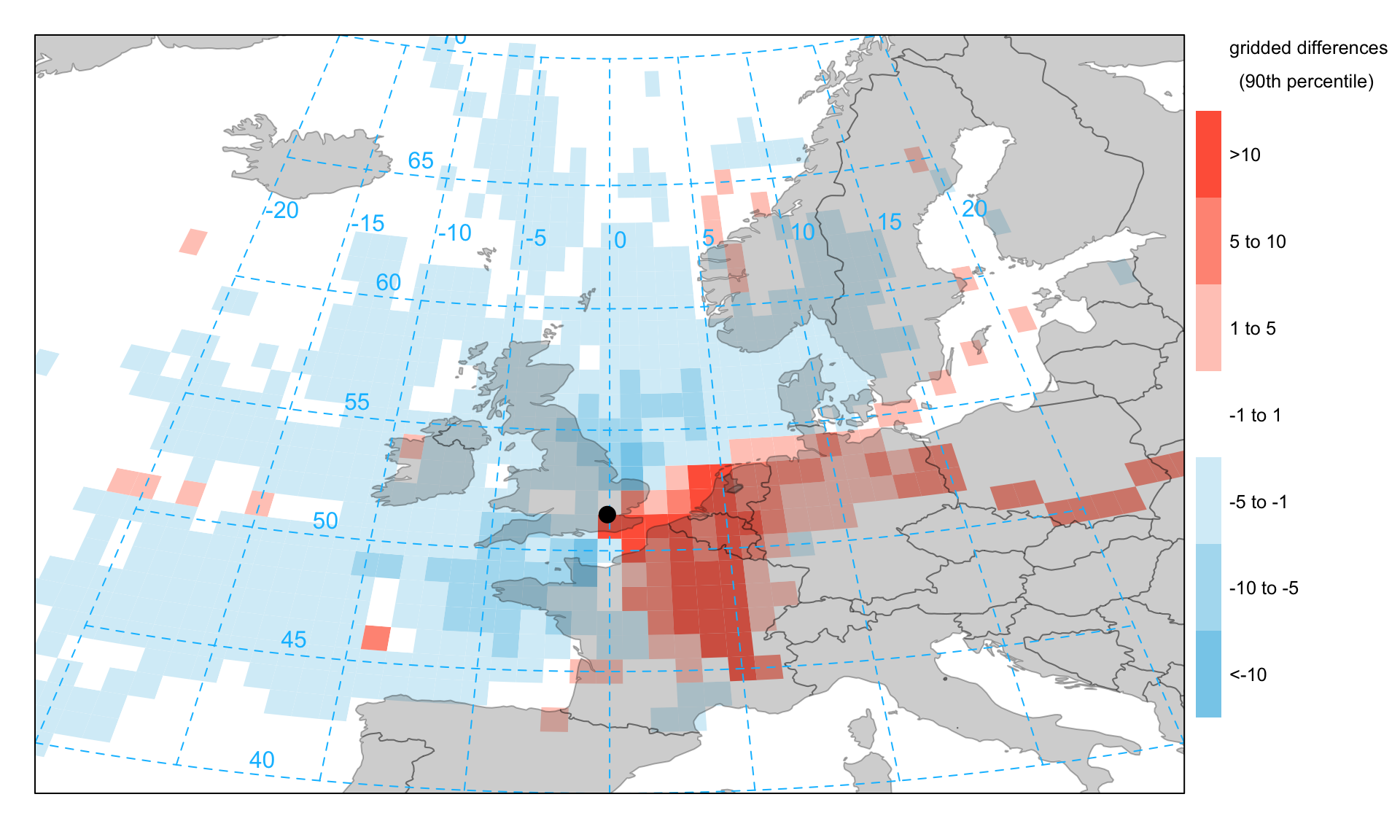
Note that it is also possible to use conditioning with these plots. For example to split the frequency results by season:
trajLevel(traj,
          pollutant = "pm10",
          statistic = "frequency",
          col = "heat",
          type = "season")
10.4.2 Allocating trajectories to different wind sectors
One of the key aspects of trajectory analysis is knowing something about where air masses have come from. Cluster analysis can be used to group trajectories based on their origins and this is discussed in Section 10.8. A simple approach is to consider different wind sectors e.g. N, NE, E and calculate the proportion of time a particular back trajectory resides in a specific sector. It is then possible to allocate a particular trajectory to a sector based on some assumption about the proportion of time it is in that sector — for example, assume a trajectory is from the west sector if it spends at least 50% of its time in that sector or otherwise record the allocation as ‘unallocated’. The code below can be used as the basis of such an approach.
First we import the trajectories, which in this case are for London in 2010:
traj <- importTraj(site = "london", year = 2010)alloc <- traj
id <- which(alloc$hour.inc == 0)
y0 <- alloc$lat[id[1]]
x0 <- alloc$lon[id[1]]
## calculate angle and then assign sector
alloc <- mutate(
alloc,
angle = atan2(lon - x0, lat - y0) * 360 / 2 / pi,
angle = ifelse(angle < 0, angle + 360 , angle),
sector = cut(angle,
breaks = seq(22.5, 382.5, 45),
labels = c("NE", "E", "SE",
"S", "SW", "W",
"NW", "N")),
sector = as.character(sector),
sector = ifelse(is.na(sector), "N", sector)
)
alloc <- group_by(alloc, date, sector) %>%
mutate(n = n()) %>%
group_by(date) %>%
arrange(date, n) %>%
slice_tail(n = 1) %>%
mutate(sector = ifelse(n > 50, sector, "unallocated")) %>%
select(date, sector, n)
# combine with trajectories
traj <- left_join(traj, alloc, by = "date")Now it is possible to post-process the data. traj now has the angle, sector and allocation (sector).
head(traj) receptor year month day hour hour.inc lat lon height pressure
1 1 2010 1 1 9 0 51.500 -0.100 10.0 994.7
2 1 2010 1 1 8 -1 51.766 0.057 10.3 994.9
3 1 2010 1 1 7 -2 52.030 0.250 10.5 995.0
4 1 2010 1 1 6 -3 52.295 0.488 10.8 995.0
5 1 2010 1 1 5 -4 52.554 0.767 11.0 995.4
6 1 2010 1 1 4 -5 52.797 1.065 11.3 995.6
date2 date sector n
1 2010-01-01 09:00:00 2010-01-01 09:00:00 unallocated 9
2 2010-01-01 08:00:00 2010-01-01 09:00:00 unallocated 9
3 2010-01-01 07:00:00 2010-01-01 09:00:00 unallocated 9
4 2010-01-01 06:00:00 2010-01-01 09:00:00 unallocated 9
5 2010-01-01 05:00:00 2010-01-01 09:00:00 unallocated 9
6 2010-01-01 04:00:00 2010-01-01 09:00:00 unallocated 9First, merge the air quality data from North Kensington:
traj <- left_join(traj, kc1, by = "date")We can work out the mean concentration by allocation, which shows the clear importance for the east and south-east sectors.
# A tibble: 9 × 2
  sector      PM2.5
  <chr>       <dbl>
1 E            21.6
2 N            11.8
3 NE           12.6
4 NW           13.6
5 S            14.5
6 SE           28.7
7 SW           10.8
8 W            11.8
9 unallocated  15.5
Finally, the percentage of the year in each sector can be calculated as follows:
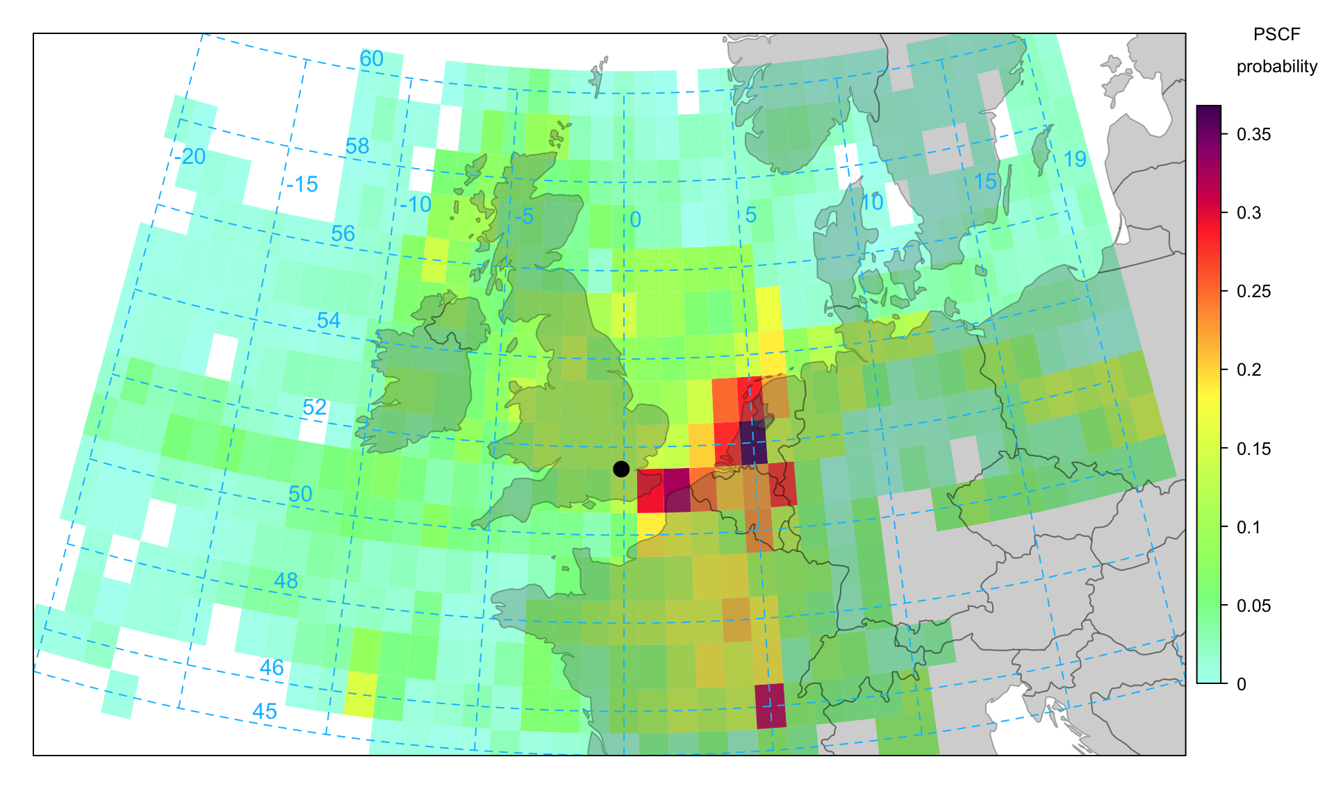
10.5 Potential Source Contribution Function (PSCF)
If statistic = "pscf" then the Potential Source Contribution Function (PSCF) is plotted. The PSCF calculates the probability that a source is located at latitude \(i\) and longitude \(j\) (Fleming et al., 2012; Pekney et al., 2006). The PSCF is somewhat analogous to the CPF function described on Section 7.3 that considers local wind direction probabilities. In fact, the two approaches have been shown to work well together (Pekney et al., 2006). The PSCF approach has been widely used in the analysis of air mass back trajectories. (Ara Begum et al., 2005) for example assessed the method against the known locations of wildfires and found it performed well for PM2.5, EC (elemental carbon) and OC (organic carbon) and that other (non-fire related) species such as sulphate had different source origins. The basis of PSCF is that if a source is located at (\(i\), \(j\)), an air parcel back trajectory passing through that location indicates that material from the source can be collected and transported along the trajectory to the receptor site. PSCF solves
\[ PSCF = \frac{m_{ij}}{n_{ij}} \tag{10.1}\]
where \(n_{ij}\) is the number of times that the trajectories passed through the cell (\(i\), \(j\)) and \(m_{ij}\) is the number of times that a source concentration was high when the trajectories passed through the cell (\(i\), \(j\)). The criterion for determining \(m_{ij}\) is controlled by percentile, which by default is 90. Note also that cells with few data have a weighting factor applied to reduce their effect.
An example of a PSCF plot is shown in Figure 10.8 for PM2.5 for concentrations 90th percentile. This Figure gives a very clear indication that the principal (high) sources are dominated by source origins in mainland Europe — particularly around the Benelux countries.
10.6 Concentration Weighted Trajectory (CWT)
A limitation of the PSCF method is that grid cells can have the same PSCF value when sample concentrations are either only slightly higher or much higher than the criterion (Hsu et al., 2003). As a result, it can be difficult to distinguish moderate sources from strong ones. (Seibert et al., 1994) computed concentration fields to identify source areas of pollutants. This approach is sometimes referred to as the CWT or CF (concentration field). A grid domain was used as in the PSCF method. For each grid cell, the mean (CWT) or logarithmic mean (used in the Residence Time Weighted Concentration (RTWC) method) concentration of a pollutant species was calculated as follows:
\[ ln(\overline{C}_{ij}) = \frac{1}{\sum_{k=1}^{N}\tau_{ijk}}\sum_{k=1}^{N}ln(c_k)\tau_{ijk} \tag{10.2}\]
where \(i\) and \(j\) are the indices of grid, \(k\) the index of trajectory, \(N\) the total number of trajectories used in analysis, \(c_k\) the pollutant concentration measured upon arrival of trajectory \(k\), and \(\tau_{ijk}\) the residence time of trajectory \(k\) in grid cell (\(i\), \(j\)). A high value of \(\overline{C}_{ij}\) means that, air parcels passing over cell (\(i\), \(j\)) would, on average, cause high concentrations at the receptor site.
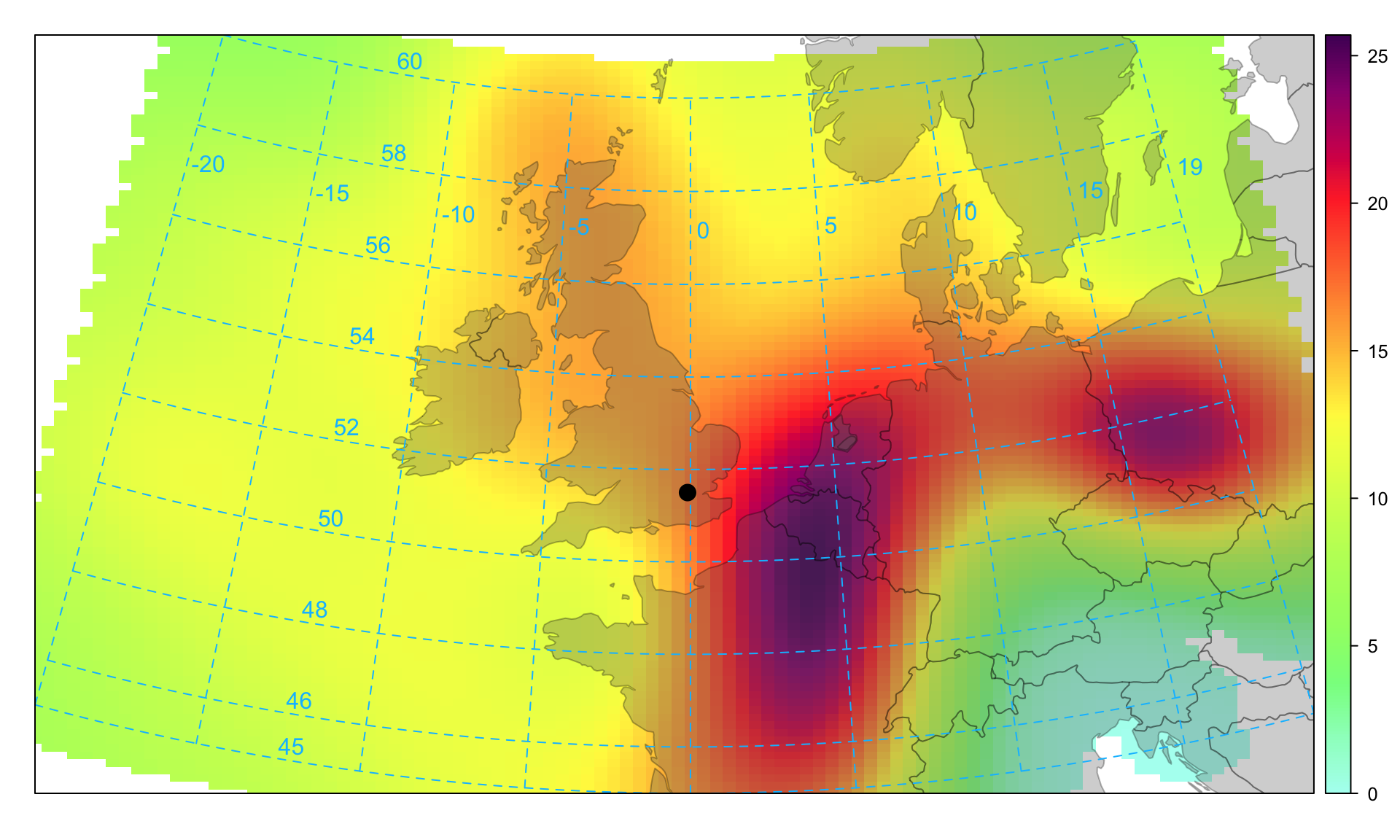
Figure 10.9 shows the situation for PM2.5 concentrations. It was calculated by recording the associated PM2.5 concentration for each point on the back trajectory based on the arrival time concentration using 2010 data. The plot shows the geographic areas most strongly associated with high PM2.5 concentrations i.e. to the east in continental Europe. Both the CWT and PSCF methods have been shown to give similar results and each have their advantages and disadvantages (Hsu et al., 2003; Lupu and Maenhaut, 2002). Figure 10.9 can be compared with Figure 10.8 to compare the overall identification of source regions using the CWT and PSCF techniques. Overall the agreement is good in that similar geographic locations are identified as being important for PM2.5.
filter(traj, lon > -20, lon < 20, lat > 45, lat < 60) %>%
  trajLevel(
    pollutant = "pm2.5",
    statistic = "cwt",
    col = "increment",
    border = "white"
  )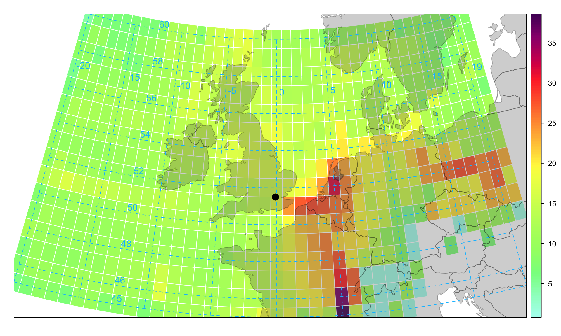
Figure 10.9 is useful, but it can be clearer if the trajectory surface is smoothed, which has been done for PM2.5 concentrations shown in Figure 10.10.
filter(traj, lat > 45 & lat < 60 & lon > -20 & lon < 20) %>%
  trajLevel(
    pollutant = "pm2.5",
    statistic = "cwt",
    smooth = TRUE,
    col = "increment"
  )
In common with most other openair functions, the flexible type option can be used to split the data in different ways. For example, to plot the smoothed back trajectories for PM2.5 concentrations by season.
It should be noted that it makes sense to analyse back trajectories for pollutants that have a large regional component — such as particles or O3. It makes little sense to analyse pollutants that are known to have local impacts e.g. NOx However, a species such as NOx can be helpful to exclude ‘fresh’ emissions from the analysis.
10.7 Simplified Quantitative Transport Bias Analysis (SQTBA)
Both CWT and PSCF techniques is essence assume that the trajectory paths represent a good estimate of the centreline of the air mass origin. However, trajectory analysis is implicitly uncertain, not least because of the difficulty of accurately describing the dispersion of pollutants in the atmosphere. Hysplit has many approaches to deal with these uncertainties such as running an ensemble of trajectories with different starting locations. However, for longer term analysis it can be very time consuming to run the model to explore the influence of meteorological variation.
SQTBA is an approach that recognises the natural processes of plume dispersion and uses this understanding as part of back trajectory analysis. The approach has been used in many studies that aim to better understand sources regions for PM2.5 (or components of PM2.5) e.g. Brook et al. (2004) considering PM2.5 in North America, Zhao et al. (2007) modelling particulate nitrate and sulphate, Zhou (2004) comparing different source attribution techniques including SQTBA and the consideration of sources of ammonia in New York State (Zhou et al., 2019).
The basic idea, only described briefly here, is that there is a natural transport behaviour of dispersing air masses that can be described by the Gaussian plume equation. Rather than a single back trajectory being considered, it is assumed that concentrations are represented according to Gaussian plume dilution along each trajectory — giving a probability of a certain concentration at a particular point on a grid. In effect, the further from a receptor (measurement site), the wider the plume (σ value), which has the effect of spreading-out the likely origin of the source. This approach is an effective, pragmatic solution to better account for the uncertainties in the location of upwind sources.
Q(x,t| x’, t’), is the probability for the air parcel at position x’ at time t’ to arrive at position x at time t is given by:
\[ Q(x, t, x', t') = \frac{1}{2 \pi \sigma_x(t') \sigma_y(t')}e^{-\frac{1}{2}\Bigg[\bigg(\frac{X - x'(t')}{\sigma_x(t')}\bigg)^2 + \bigg(\frac{Y - y'(t')}{\sigma_y(t')}\bigg)^2\Bigg]} \]
X, Y: Coordinate of the grid centre
x’ y’: Centreline of trajectory
σ: Standard deviation of trajectories at two directions which are assumed to grow with time
σx(t’) = σy(t’) = at’, a is a dispersion speed, equals to 1.5 km h-1. Note that the default σ is assumed to be 1.5 km h-1 rather than 5.4 km h-1 that is commonly used in other studies because testing shows that a lower value reveals more information about source origins without introducing noise. In practice, the value of σ will vary depending on meteorological conditions and be influenced by both turbulence and wind shear. Users can set their own value of σ in the function options.
This means at each trajectory point, the probability is calculated across a pre-defined grid. These calculations can take some time to run. For example, with 96 hour back trajectories calculated every 3 hours in a year, there are 840,960 trajectory end points. Each one of these points is used to estimate the probability on a grid, which itself can be large (a one degree grid from 35 to 80°N and -55 to 25°W is 3600 grid points).
A potential mass transfer field is calculated for a given trajectory l, arriving at time t, is integrated over back trajectory time 𝜏:
\[ \overline{T_l}(x | x') = \frac{\int_{t-\tau}^{t} Q(x,t| x', t')dt'}{\int_{t-\tau}^{t}dt'} \]
and the concentration-weighted field calculated as:
\[ \widetilde{T}(x|x') = \sum_{l=1}^{l=L}\overline{T_l}(x|x')c_l \]
cl: Receptor concentration of back trajectory l
L: Total number of back trajectories
And the final SQTBA is calculated as:
\[ SQTBA(x|x') = \frac{\widetilde{T}(x|x')}{\sum_{l=1}^{l=L}\overline{T_l}(x|x')} \]
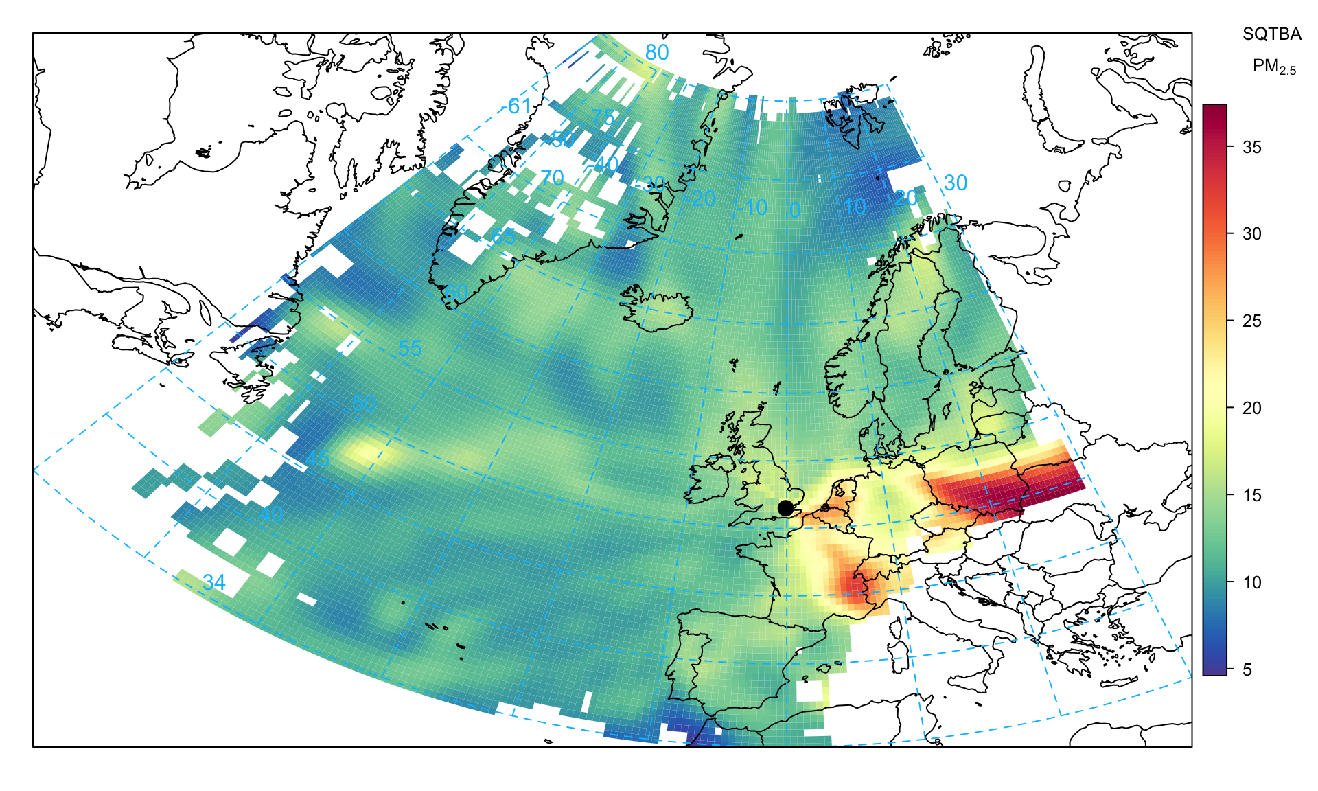
As an example, consideration is given to PM2.5 concentrations in a similar way as shown for CWT and the PSCF techniques. This plot indicates several potential sources of PM2.5 precursors with the Benelux countries and around the Po Valley in Italy (known high NOx emission regions and potential sources of ammonium nitrate), and also a higher source region in eastern Europe across south Poland.
trajLevel(
  dplyr::slice_sample(traj, prop = 0.1),
  pollutant = "pm2.5",
  statistic =  "sqtba",
  map.fill = FALSE,
  cols = "default",
  lat.inc = 0.5,
  lon.inc = 0.5
)
Some further analysis can be carried out on the TEOM FDMS measurements, which separately reports the volatile and non-volatile components of PM. Figure 10.12 shows the plot for the volatile PM2.5 component, which highlights the source regions of the Benelux counties and (likely) northern Italy.
trajLevel(traj,
          pollutant = "v2.5",
          statistic =  "sqtba",
          map.fill = FALSE,
          cols = "default",
          lat.inc = 0.5,
          lon.inc = 0.5
          )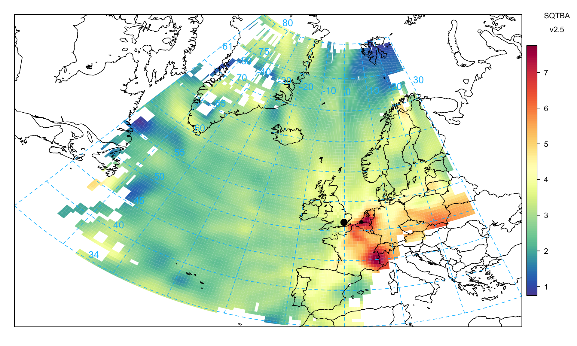
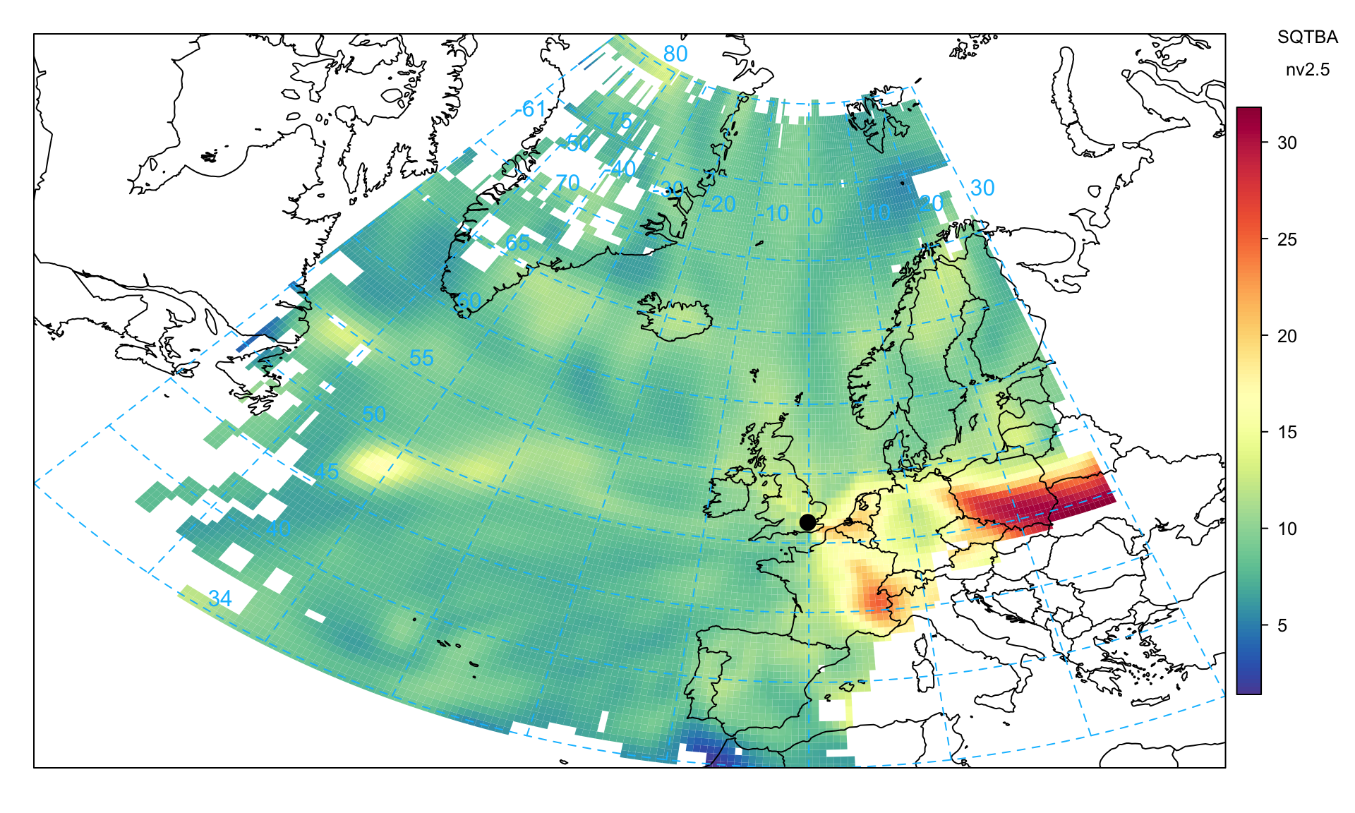
On the other hand, Figure 10.13 shows the non-volatile PM2.5 component, which more clearly shows eastern Europe as the principal source. This plot differs from Figure 10.12 and likely highlights the higher sulphur emissions from power generation in this part of Europe. More detailed analysis can be carried out if the components of PM are available at an hourly or daily resolution e.g. particulate nitrate, sulphate.
trajLevel(
  traj,
  pollutant = "nv2.5",
  statistic =  "sqtba",
  map.fill = FALSE,
  cols = "default",
  lat.inc = 0.5,
  lon.inc = 0.5
)
The analysis above was demonstrated for a single site. However, to exploit the full potential of the SQTBA approach, multiple receptors should be considered. The reason why multiple sites should be considered is that there will be better geographic coverage of the trajectories and potential for source regions to be sampled multiple times. To conduct an analysis of multiple sites, trajectories linked to pollutant concentrations should be combined into a single data frame in the format similar to traj above but with an additional variable that identifies the different sites. When running trajLevel the option .combine should be used to identify the relevant column e.g. .combine = "site".
The results returned from multiple site analysis are normalised by each site individually by dividing the output by the mean of the pollutant concentration. This approach ensures that sites with potentially very different mean concentrations can be used in a consistent way to identify source regions, without single sites dominating the output.
10.8 Trajectory clustering
Often it is useful to use cluster analysis on back trajectories to group similar air mass origins together. The principal purpose of clustering back trajectories is to post-process data according to cluster origin. By grouping data with similar geographic origins it is possible to gain information on pollutant species with similar chemical histories. There are several ways in which clustering can be carried out and several measures of the similarity of different clusters. A key issue is how the distance matrix is calculated, which determines the similarity (or dissimilarity) of different back trajectories. The simplest measure is the Euclidean distance. However, an angle-based measure is also often used. The two distance measures are defined below. In openair the distance matrices are calculated using C\(++\) code because their calculation is computationally intensive. Note that these calculations can also be performed directly in the Hysplit model itself.
The Euclidean distance between two trajectories is given by Equation 10.3. Where \(X_1\), \(Y_1\) and \(X_2\), \(Y_2\) are the latitude and longitude coordinates of back trajectories \(1\) and \(2\), respectively. \(n\) is the number of back trajectory points (96 hours in this case). Note that a simpler formula is sufficient for this calculation than the more accurate Haversine formula.
\[ d_{1, 2} = \left({\sum_{i=1}^{n} 111((X_{1i} - X_{2i}) ^ 2 + ((Y_{1i} - Y_{2i})cos(X_{1i})) ^ 2}\right)^{1/2} \tag{10.3}\]
The angle distance matrix is a measure of how similar two back trajectory points are in terms of their angle from the origin i.e. the starting location of the back trajectories. The angle-based measure will often capture some of the important circulatory features in the atmosphere e.g. situations where there is a high pressure located to the east of the UK. However, the most appropriate distance measure will be application dependent and is probably best tested by the extent to which they are able to differentiate different air-mass characteristics, which can be tested through post-processing. The angle-based distance measure is defined as:
\[ d_{1, 2} = \frac{1}{n}\sum_{i=1}^{n}cos^{-1} \left(0.5\frac{A_i + B_i - C_i}{\sqrt{A_iB_i}}\right) \tag{10.4}\]
where
\[ A_i = (X_1(i) - X_0)^2 + (Y_1(i) - Y_0)^2 \tag{10.5}\]
\[ B_i = (X_2(i) - X_0)^2 + (Y_2(i) - Y_0)^2 \tag{10.6}\]
\[ C_i = (X_2(i) - X_1(i))^2 + (Y_2(i) - Y_1(i))^2 \tag{10.7}\]
where \(X_0\) and \(Y_0\) are the coordinates of the location being studied i.e. the starting location of the trajectories.
As an example we will consider back trajectories for London in 2011.
First, the back trajectory data for London is imported together with the air pollution data for the North Kensington site (KC1).
traj <- importTraj(site = "london", year = 2011)
kc1 <- importUKAQ(site = "kc1", year = 2011)
The clusters are straightforward to calculate. In this case the back trajectory data (traj) is supplied and the angle-based distance matrix is used. Furthermore, we choose to calculate 6 clusters and choose a specific colour scheme. In this case we read the output from trajCluster into a variable clust so that the results can be post-processed.
clust <- trajCluster(traj, method = "Angle",
                     n.cluster = 6,
                     col = "Set2",
                     map.cols = openColours("Paired", 10))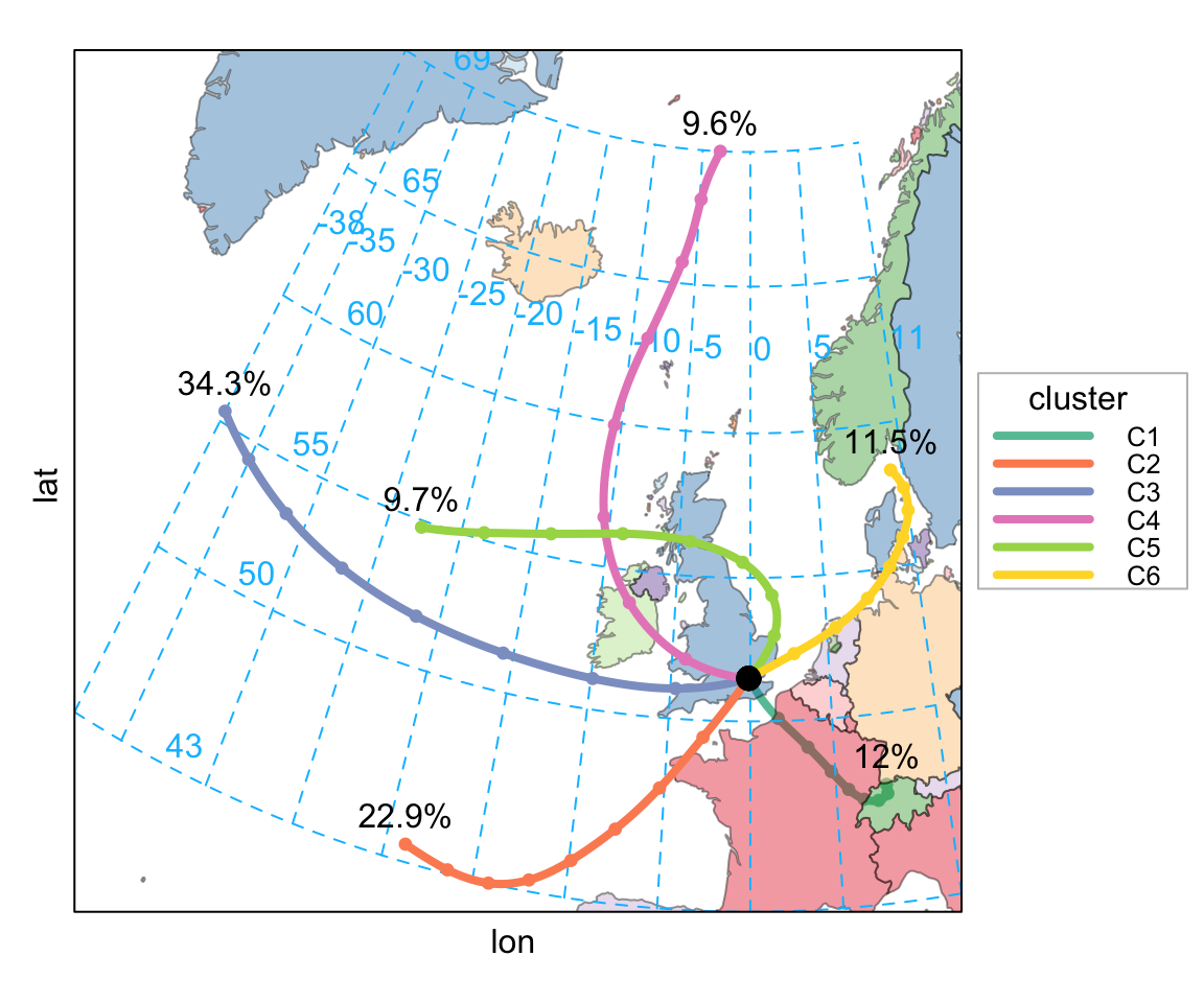
clust returns all the back trajectory information together with the cluster (as a character). This data can now be used together with other data to analyse results further. However, first it is possible to show all trajectories coloured by cluster, although for a year of data there is significant overlap and it is difficult to tell them apart.
trajPlot(clust$data$traj, group = "cluster")A useful way in which to see where these air masses come from by trajectory is to produce a frequency plot by cluster. Such a plot (not shown, but code below) provides a good indication of the spread of the different trajectory clusters as well as providing an indication of where air masses spend most of their time. For the London 2011 data it can be seen cluster 1 is dominated by air from the European mainland to the south.
trajLevel(clust$data$traj, type = "cluster",
          col = "increment",
          border = NA)
Perhaps more useful is to merge the cluster data with measurement data. In this case the data at North Kensington site are used. Note that in merging these two data frames it is not necessary to retain all 96 back trajectory hours and for this reason we extract only the first hour.
# use inner join - so only where we have data in each
kc1 <- inner_join(kc1,
                  filter(clust$data$traj, hour.inc == 0),
                  by = "date")
Now kc1 contains air pollution data identified by cluster. The size of this data frame is about a third of the original size because back trajectories are only run every 3 hours.
The numbers of each cluster are given by:
table(kc1[["cluster"]])
 C1  C2  C3  C4  C5  C6
347 661 989 277 280 333
i.e. is dominated by clusters 3 and 2 from west and south-west (Atlantic).
Now it is possible to analyse the concentration data according to the cluster. There are numerous types of analysis that can be carried out with these results, which will depend on what the aims of the analysis are in the first place. However, perhaps one of the first things to consider is how the concentrations vary by cluster. As the summary results below show, there are distinctly different mean concentrations of most pollutants by cluster. For example, clusters 1 and 6 are associated with much higher concentrations of PM10 — approximately double that of other clusters. Both of these clusters originate from continental Europe. Cluster 5 is also relatively high, which tends to come from the rest of the UK. Other clues concerning the types of air-mass can be gained from the mean pressure. For example, cluster 5 is associated with the highest pressure (1014 kPa), and as is seen in Figure 10.14 the shape of the line for cluster 5 is consistent with air-masses associated with a high pressure system (a clockwise-type sweep).
# A tibble: 6 × 28
  cluster    co   nox   no2    no    o3   so2  pm10 pm2.5   v10  v2.5  nv10
  <chr>   <dbl> <dbl> <dbl> <dbl> <dbl> <dbl> <dbl> <dbl> <dbl> <dbl> <dbl>
1 C1      0.346  89.9  51.4 25.3   32.1  3.12  38.3  31.3  8.79  8.02  29.5
2 C2      0.205  40.9  30.9  6.55  39.4  1.46  17.2  11.6  4.18  3.13  13.1
3 C3      0.198  47.2  32.3  9.78  39.7  1.84  18.1  11.3  3.73  2.80  14.3
4 C4      0.189  44.1  30.6  8.89  39.7  1.56  17.8  11.0  3.41  2.17  14.4
5 C5      0.202  57.0  39.2 11.7   41.4  2.31  24.3  16.5  5.06  4.50  19.2
6 C6      0.267  64.9  42.4 14.8   46.3  2.93  36.6  29.7  7.78  7.57  28.8
# ℹ 16 more variables: nv2.5 <dbl>, ws <dbl>, wd <dbl>, air_temp <dbl>,
#   receptor <dbl>, year <dbl>, month <dbl>, day <dbl>, hour <dbl>,
#   hour.inc <dbl>, lat <dbl>, lon <dbl>, height <dbl>, pressure <dbl>,
#   traj_len <dbl>, len <dbl>
Simple plots can be generated from these results too. For example, it is easy to consider the temporal nature of the volatile component of PM2.5 concentrations (v2.5 in the kc1 data frame). Figure 10.15 for example shows how the concentration of the volatile component of PM2.5 concentrations varies by cluster by plotting the hour of day-month variation. It is clear from Figure 10.15 that the clusters associated with the highest volatile PM2.5 concentrations are clusters 1 and 6 (European origin) and that these concentrations peak during spring. There is less data to see clearly what is going on with cluster 5. Nevertheless, the cluster analysis has clearly separated different air mass characteristics which allows for more refined analysis of different air-mass types.
trendLevel(kc1, pollutant = "v2.5", type = "cluster",
           layout = c(6, 1),
               cols = "increment")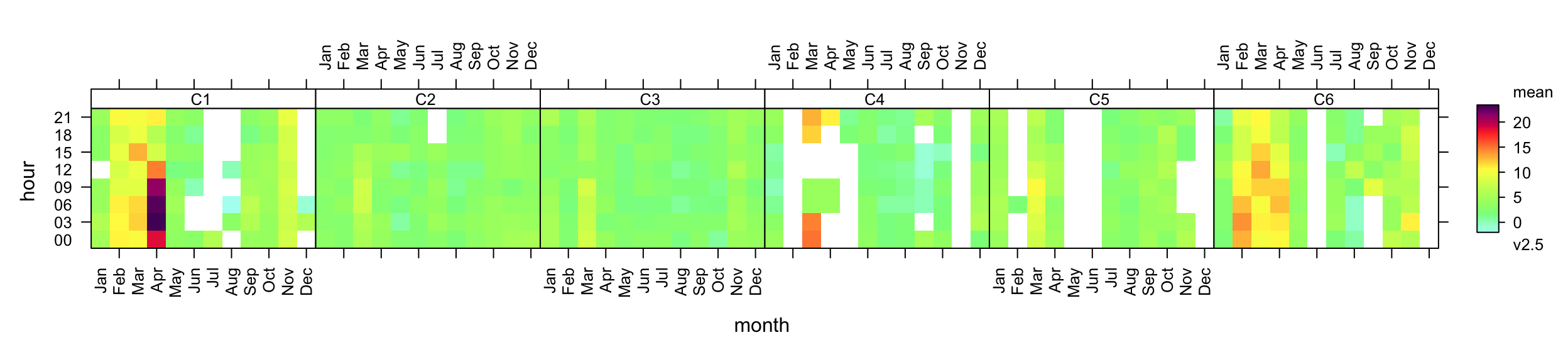
Similarly, as considered in Section 8.8, the timeVariation function can also be used to consider the temporal components.
Another useful plot to consider is timeProp (see Chapter 14), which can show how the concentration of a pollutant is comprised. In this case it is useful to plot the time series of PM2.5and show how much of the concentration is contributed to by each cluster. Such a plot is shown in Figure 10.16. It is now easy to see for example that during the spring months many of the high concentration events were due to clusters 1 and 6, which correspond to European origin air-masses as shown in Figure 10.14.
timeProp(kc1, pollutant = "pm2.5",
         avg.time = "day", proportion = "cluster",
         cols = "Set2",
         key.position = "top", key.columns = 6)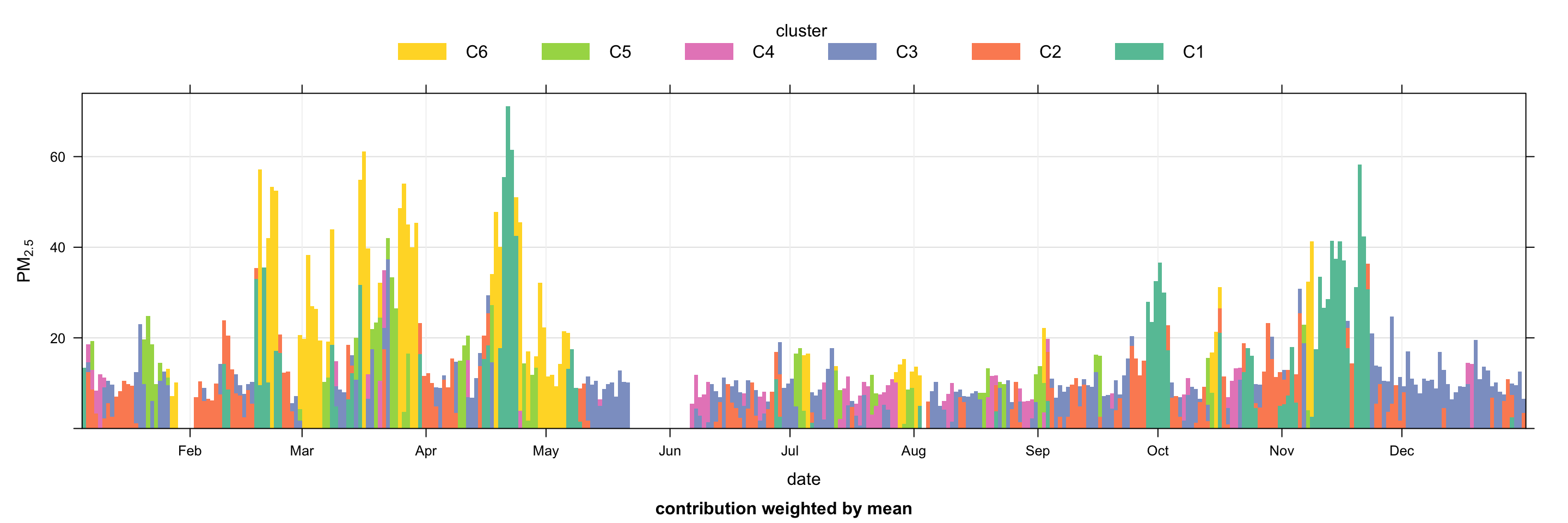
10.9 Trajectories on an interactive map
An R package called openairmaps has been developed to plot trajectories on interactive leaflet maps. This package can be installed from CRAN, similar to openair.
install.packages("openairmaps")The function trajMap is the openairmaps equivalent of the trajPlot function. The package comes with some example data (traj_data) that can be used as a template for using other importTraj outputs.
First, load the package.
Plot an interactive map. Try clicking on the individual
trajMap(traj_data, colour = "pm10")Interactive map of trajectories with the default map.
The trajMap function allows for control of many parts of the leaflet map. For example, you can provide one (or more) different base map(s) — there are many! You can also specify a “control” column, which will allow you to show and hide certain trajectory paths. This is nicely showcased using output from the trajCluster function.
clustdata <- trajCluster(traj_data)trajMap(
data = clustdata$data$traj,
colour = "cluster",
control = "cluster",
provider = "CartoDB.Positron"
)Interactive map of clustered trajectories on a new basemap.
openairmaps also contains an equivalent to trajLevel. trajlevelMap takes many of the same arguments as trajLevel and works with all statistic types, but returns an interactive map. Try hovering over and clicking on the tiles.
trajLevelMap(traj_data, statistic = "frequency")An interactive ‘frequency’ map plotted by trajLevelMap.
For more information about using openairmaps to visualise trajectories, please refer to the Interactive Trajectory Analysis Page.
Note — the back trajectories have been pre-calculated for specific locations and stored as .RData objects. Users should contact David Carslaw to request the addition of other locations.↩︎
You will need to load the mapdata package i.e.
library(mapdata).↩︎