Chapter 8 Taylor’s Theorem

8.1 Recap of Taylor’s Theorem for $f(x)$

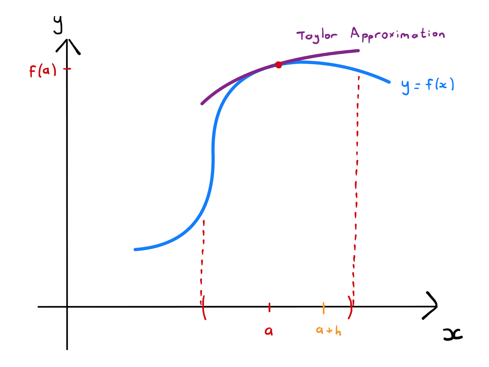
Taylor’s Theorem: Let $f(x)$ be a univariate real-valued function that is infinitely differentiable and let $a \in \mathbb{R}$. For sufficiently small values of $h$, one has $$f(a+h) = \sum\limits_{r=0}^{n} \frac{1}{r!} h^{r} f^{(r)}(a) + R_n$$ where the remainder $R_n$ is given by $$R_n = \frac{1}{(n+1)!} h^{n+1} f^{(n+1)}(a+th), \qquad \text{for some } t \in [0,1].$$

Note that $R_n$ is the next term that would appear in the summation only with $(n+1)^{th}$ derivative of $f$ evaluated at some unknown value between $a$ and $a+h$.

The expression $\sum\limits_{r=0}^{n} \frac{1}{r!} h^{r} f^{(r)}(a)$ appearing in Taylor’s theorem is known as the $n^{th}$ Taylor polynomial of $f$ about $a$.

Treating $h$ as a variable, the $n^{th}$ Taylor polynomial is indeed a polynomial of degree $n$. Since $h = x-a$ where $a$ is fixed, the $n^{th}$ Taylor polynomial can be thought of as a polynomial in $x$ of degree $n$. The idea is that the Taylor polynomials give a polynomial approximation of $f(x)$ in a neighborhood of $a$ which in general improves with increasing $n$.

Let $n \rightarrow \infty$ in Taylor’s Theorem. If $R_{n} \rightarrow 0$ and $h$ is substituted for $x-a$, then one obtains the Taylor series of $f$ about $a$: $$\begin{align*} f(x) &= f(a) + (x-a) f'(a) + \frac{1}{2}(x-a)^2 f''(a) + \ldots + \frac{1}{n!} (x-a)^{n} f^{(n)}(a) + \ldots \\ &= \sum\limits_{r=0}^{\infty} \frac{1}{k!} (x-a)^{r} f^{(r)}(a). \end{align*}$$

Taking $a=0$ in Definition 8.1.3 recovers the MacClaurin series of $f(x)$.

8.2 Taylor’s Theorem for $f(x,y)$

Taylor’s Theorem extends to multivariate functions. In particular we will study Taylor’s Theorem for a function of two variables.

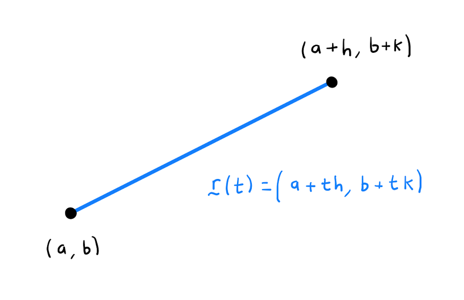
Taylor’s Theorem: Let $f(x,y)$ be a real-valued function of two variables that is infinitely differentiable and let $(a,b) \in \mathbb{R}^{2}$. For sufficiently small values of $h,k$, one has $$f(a+h,b+k) = \sum\limits_{r=0}^{n} \frac{1}{r!} \left. \left( (x-a) \frac{\partial}{\partial x} + (y-b) \frac{\partial}{\partial y} \right)^{r} f(x,y) \right\rvert_{(a,b)} + R_n$$ where the remainder $R_n$ is given by $$R_n = \frac{1}{(n+1)!} \left. \left( h \frac{\partial}{\partial x} + k \frac{\partial}{\partial y} \right)^{n+1} f(x,y) \right\rvert_{(a+th,b+tk)}, \qquad \text{for some } t \in [0,1].$$

Note that the expression $h \frac{\partial}{\partial x} + k \frac{\partial}{\partial y}$ appearing in Theorem 8.2.1 is an operator that will be applied to $f(x,y)$. For example $$\left( h \frac{\partial}{\partial x} + k \frac{\partial}{\partial y} \right) f(x,y) = h \frac{\partial f}{\partial x} + k \frac{\partial f}{\partial y}.$$ The exponent $r$ of this operator dictates that the operator should be applied $r$ times. For example $$\begin{align*} \left( h \frac{\partial}{\partial x} + k \frac{\partial}{\partial y} \right)^2 f(x,y) &=\left( h \frac{\partial}{\partial x} + k \frac{\partial}{\partial y} \right) \left( h \frac{\partial f}{\partial x} + k \frac{\partial f}{\partial y} \right) \\ &= h^2 \frac{\partial^2 f}{\partial x^2} + 2hk \frac{\partial^2 f}{\partial x \partial y} + k^2 \frac{\partial^2 f}{\partial y^2}. \end{align*}$$ The result of this operator being applied to $f(x,y)$ is subsequently evaluated at the point $(a,b)$. This is indicated by the notation $\rvert_{(a,b)}$.

The term $R_n$ featuring in Theorem 8.2.1, is the next term that would appear in the summation except for that the $(n+1)^{th}$ partial derivatives of $f(x,y)$ are evaluated at some unknown point on the straight line between $(a,b)$ and $(a+h,b+k)$.

The exact value of $t$ is not usually known exactly, meaning the value of $R_n$ is unknown. However an upper bound on $R_n$ is often possible, meaning that the summation in Theorem 8.2.1 provides an approximation to $f(x,y)$ with a calculable accuracy.

The expression $\sum\limits_{r=0}^{n} \frac{1}{r!} \left. \left( h \frac{\partial}{\partial x} + k \frac{\partial}{\partial y} \right)^{r} f(x,y) \right\rvert_{(a,b)}$ appearing in Taylor’s theorem is known as the $n^{th}$ Taylor polynomial of $f(x,y)$ about $(a,b)$.

Treating $h$ and $k$ as variables, the $n^{th}$ Taylor polynomial is indeed a polynomial of degree $n$. Since $h = x-a, k=y-b$ where $(a,b)$ is fixed, the $n^{th}$ Taylor polynomial can be thought of as a polynomial in variables $x,y$ of degree $n$. The idea is that the Taylor polynomials give a polynomial approximation of $f(x,y)$ in a neighborhood of $(a,b)$ which in general improves with increasing $n$.

The first few terms of the sum in Taylor’s theorm grouped by degree are given explicitly by $$\begin{align*} f(a+h,b+k) = f(a,b) + \bigg( &h f_x(a,b) + k f_y(a,b) \bigg) \\ &+ \frac{1}{2} \bigg(h^2 f_{xx}(a,b) + 2hk f_{xy}(a,b) + k^2 f_{yy}(a,b) \bigg) + \ldots \end{align*}$$

Let $n \rightarrow \infty$ in Taylor’s Theorem. If $R_{n} \rightarrow 0$ and $x-a$, $y-b$ are substituted in for $h, k$ respectively, then one obtains the Taylor series of $f$ about $(a,b)$: $$\begin{align*} f(x,y) &= f(a,b) + (x-a) f_{x}(a,b) + (y-b) f_y(a,b) + \frac{1}{2}(x-a)^2 f_{xx}(a,b) + \ldots \\ &= \sum\limits_{r=0}^{\infty} \frac{1}{r!} \left. \left( h \frac{\partial}{\partial x} + k \frac{\partial}{\partial y} \right)^{r} f(x,y) \right\rvert_{(a,b)}. \end{align*}$$

8.3 Linear Approximation using Taylor’s Theorem

Having established that the $n^{th}$ Taylor polynomial from Definition 8.2.2 gives a degree $n$ polynomial approximation of $f$ in a neighbourhood of $(a,b)$, by setting $n=1$ one obtains a linear approximation of $f(x,y)$ near $(a,b)$. Specifically $$f(x,y) \approx f(a,b) + (x-a) f_{x}(a,b) + (y-b) f_y (a,b) = L(x,y).$$

Note $z=L(x,y)$ is linear in $x$ and $y$ so is a plane. Specifically this is the tangent plane to the surface $z=f(x,y)$ at $(a,b)$.

Indeed this linear approximation is one we have already seen in the course. This approximation is essentially the same as the small changes formula $\Delta f = \frac{\partial f}{\partial x} \Delta x + \frac{\partial f}{\partial y} \Delta y$ that we saw in Section 5.1.

Find the linear approximation to the function $f(x,y)= \frac{1}{2}xy + 2$ near $(x,y)=(2,1)$.

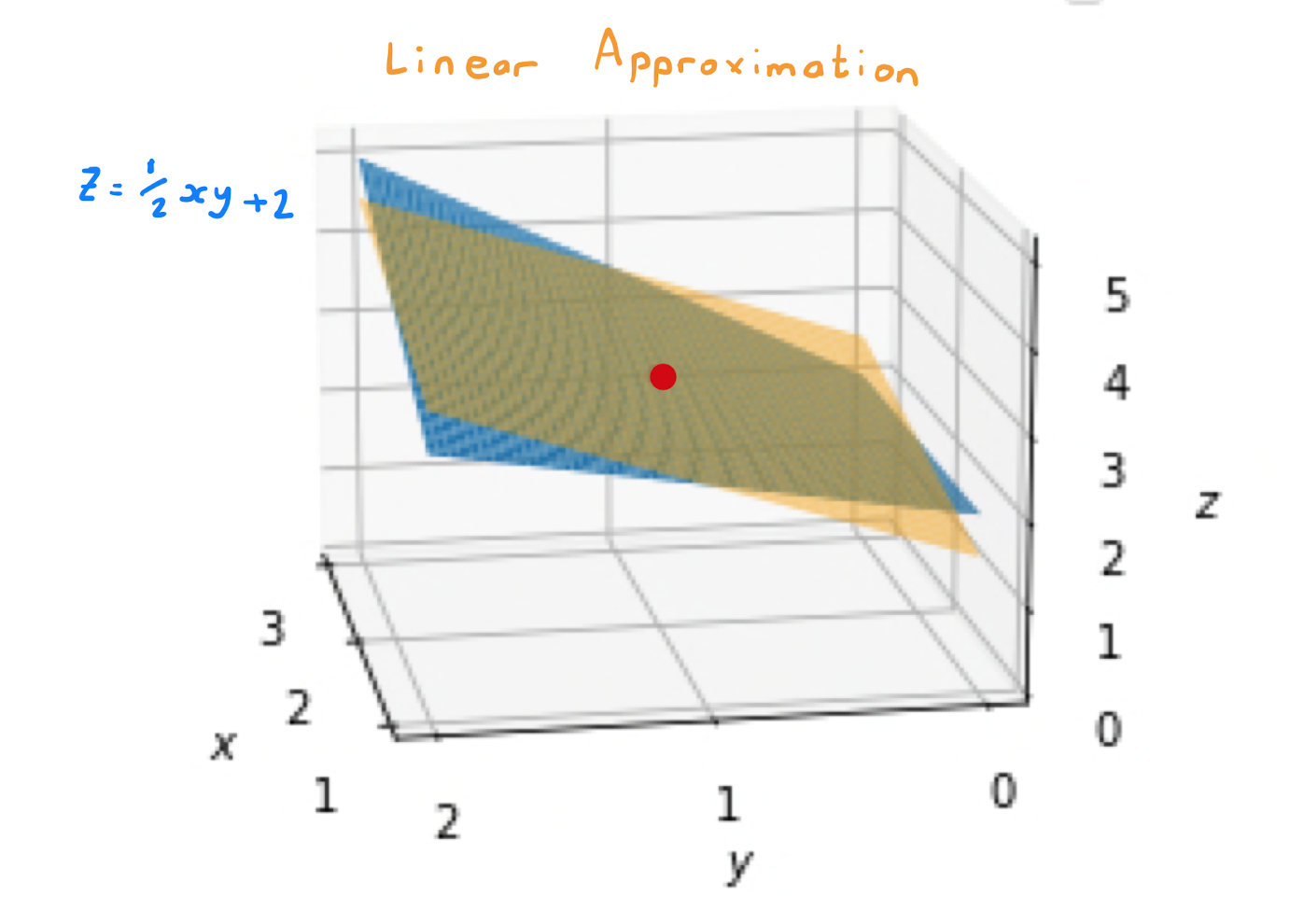
The linear approximation of $f$ obtained through Taylor’s theorem, setting $a=2, b=1$, is $$f(x,y) \approx L(x,y) = f(2,1) + (x-2) f_x (2,1) + (y-1) f_y (2,1).$$ Calculate that $$\begin{align*} &f(x,y) = \frac{1}{2}xy +2, \qquad \qquad &f(2,1) = 3, \\ &f_x(x,y) = \frac{1}{2}y, \qquad \qquad &f_x(2,1) = \frac{1}{2}, \\ &f_y(x,y) = \frac{1}{2}x, \qquad \qquad &f_y(2,1) = 1. \end{align*}$$ Therefore the required linear approximation is $$L(x,y) = 3 +\frac{1}{2} \cdot (x-2) + 1 \cdot (y-1) = \frac{1}{2}x + y+1.$$

$L(x,y)$ has the following properties:

• $L(a,b) = f(a,b)$;

• $L_x(a,b) = f_x(a,b)$;

• $L_y(a,b) = f_y(a,b)$.

Prove each of the statements in Lemma 8.3.2.

8.4 Quadratic Approximation using Taylor’s Theorem

Similarly to Section 8.3, setting $n=2$ in the Taylor polynomial of Definition 8.2.2 gives a quadratic approximation of $f$ in a neighbourhood of $(a,b)$. Specifically $$\begin{align*} f(x,y) \approx f(a,b) + &(x-a) f_x(a,b) + (y-b) f_y(a,b) \\ &+ \frac{1}{2} \Big[ (x-a)^2 f_{xx}(a,b) + 2(x-a)(y-b) f_{xy}(a,b) + (y-b)^2 f_{yy}(a,b) \Big] \\ =Q(x,y).& \end{align*}$$

Find the quadratic approximation to the function $f(x,y)= e^{x^2 +y}$ in a neighbourhood of $(0,0)$.

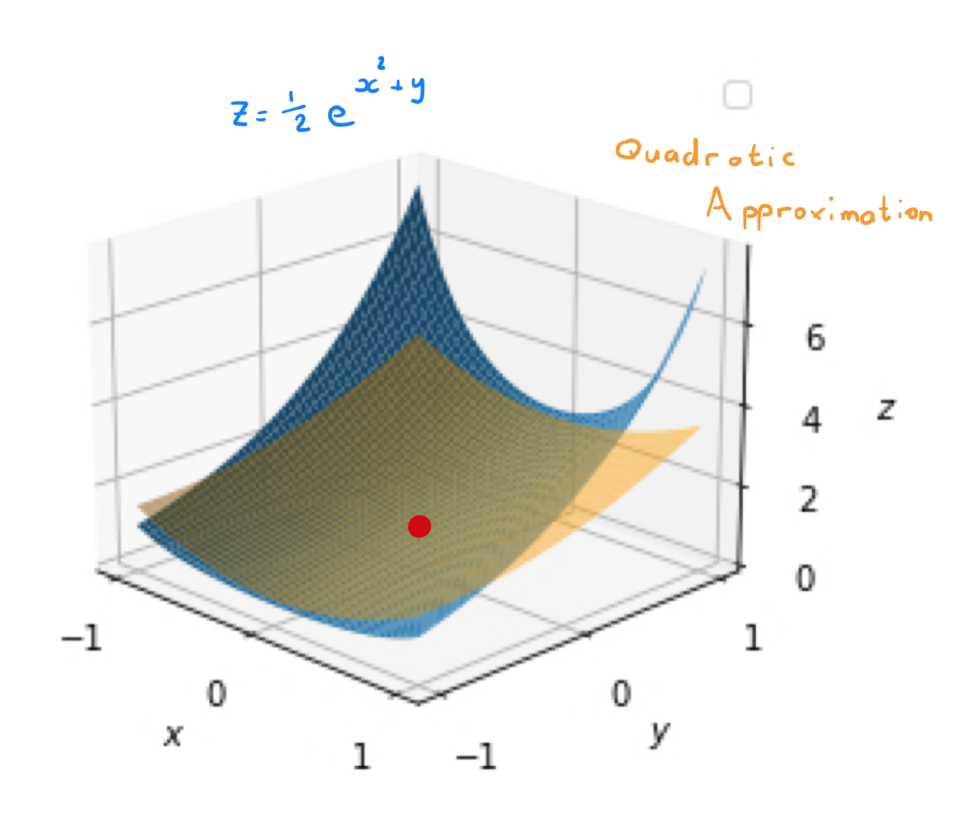
The quadratic approximation of $f$ obtained through Taylor’s theorem, setting $a=0, b=0$, is $$\begin{align*} f(x,y) &\approx Q(x,y) \\ &= f(0,0) + xf_x (0,0) + y f_y (0,0) + \frac{1}{2} \Big[ x^2 f_{xx}(0,0) + 2xy f_{xy}(0,0) + f_{yy}(0,0) \Big] \end{align*}$$

Calculate that

$$\begin{align*} &f(x,y) = e^{x^2 +y}, \qquad \qquad &f(0,0) = 1, \\ &f_{x}(x,y) = 2xe^{x^2 +y}, \qquad \qquad &f_{x}(0,0) = 0, \\ &f_{y}(x,y) = e^{x^2 +y}, \qquad \qquad &f_{y}(0,0) = 1, \\ &f_{xx}(x,y) = (2+4x^2)e^{x^2 +y}, \qquad \qquad &f_{xx}(0,0) = 2, \\ &f_{xy}(x,y) = 2xe^{x^2 +y}, \qquad \qquad &f_{xy}(0,0) = 0, \\ &f_{yy}(x,y) = e^{x^2 +y}, \qquad \qquad &f_{yy}(0,0) = 1. \end{align*}$$

Therefore the required quadratic approximation is given by

$$\begin{align*} Q(x,y) &= 1 + x \cdot 0 + y \cdot 1 + \frac{1}{2} \Big[ x^2 \cdot 2 + 2xy \cdot 0 + y^2 \cdot 1 \Big] \\ &= 1 + y+ x^2 + \frac{1}{2} y^2. \end{align*}$$

Find the quadratic approximation $Q(x,y)$ to the function $f(x,y)= \frac{1}{2}xy + 2$ near $(x,y)=(2,1)$. What do you notice about the answer?

$Q(x,y)$ has the following properties:

• $Q(a,b) = f(a,b)$;

• $Q_x(a,b) = f_x(a,b)$;

• $Q_y(a,b) = f_y(a,b)$;

• $Q_{xx}(a,b) = f_{xx}(a,b)$;

• $Q_{xy}(a,b) = f_{xy}(a,b)$;

• $Q_{yy}(a,b) = f_{yy}(a,b)$.

Prove each of the statements in Lemma 8.4.2.