Chapter 9 Stationary Points

9.1 Definition of Stationary Points

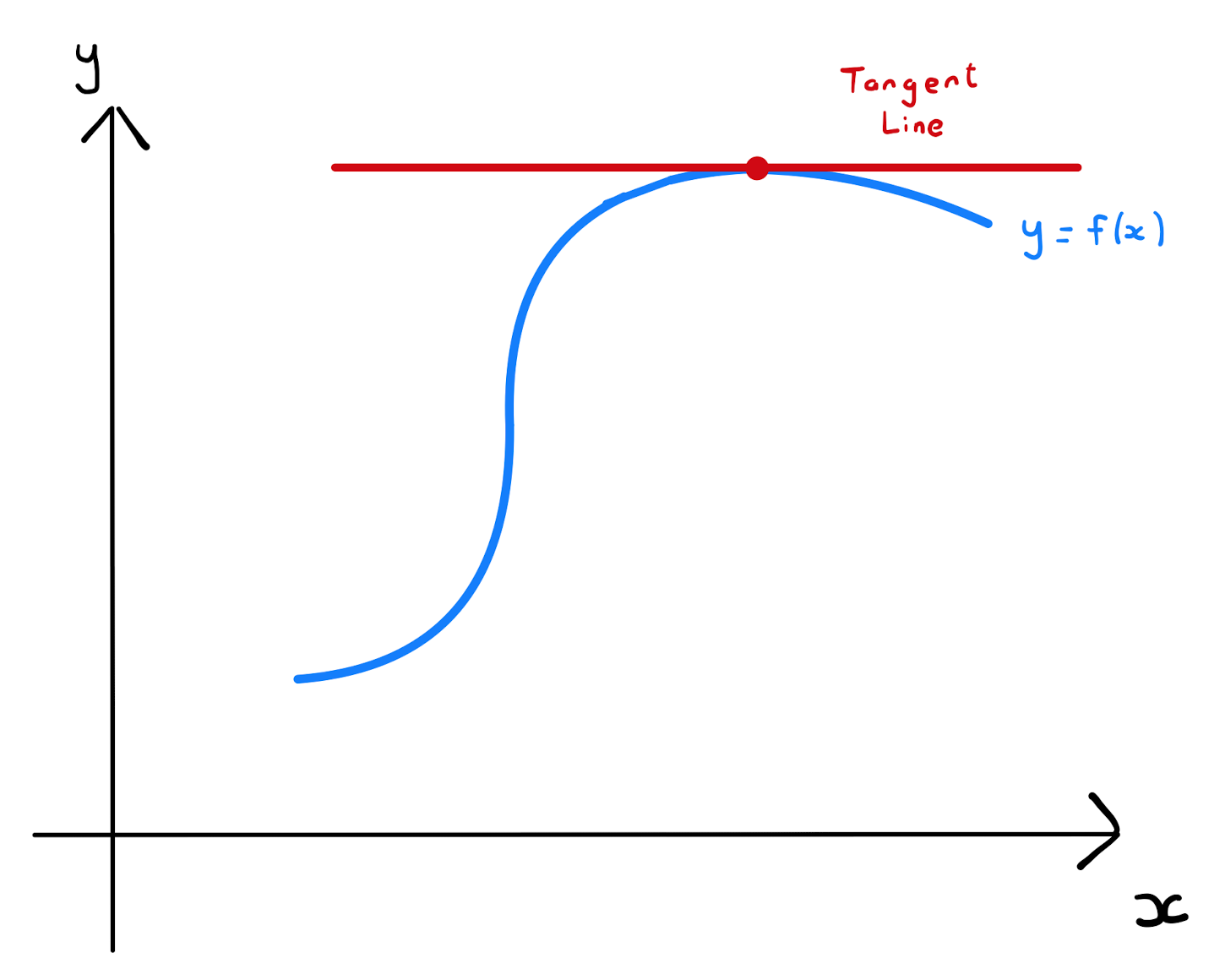
Recall that for a univariate function $y=f(x)$, a stationary point is a value $x_0$ for $x$ at which $f'(x_0)=0$. Graphically this is a point on the curve at which the tangent line is horizontal.

Now consider a function of two variables $z=f(x,y)$.

A point $(a,b)$ at which $f_x (a,b) = f_y (a,b) = 0$ is a stationary point of $f(x,y)$.

Calculate the stationary points of the function $f(x,y)=x^2 + y^2$.

Calculating the first order partial derivatives one obtains

$$\begin{align*} f_x &= 2x, \\ f_y &= 2y. \end{align*}$$

So

$$\begin{align*} &f_x = 0, \text{ and } f_y = 0 \\[5pt] \iff \qquad &2x = 0, \text{ and } 2y = 0 \\[5pt] \iff \qquad &x=0, \text{ and } y=0. \end{align*}$$

Therefore $f$ has a unique stationary point at $(0,0)$.

Calculate the stationary points of the function $f(x,y)=6 x^2 y -3x^3+ 2y^3 -150y$.

Calculating the first order partial derivatives one obtains $$\begin{align*} f_x &= 12xy - 9x^2, \\ f_y &= 6 x^2 +6 y^2 -150. \end{align*}$$ So $$\begin{align*} &f_x = 0, \text{ and } f_y = 0 \\[5pt] \iff \qquad &12xy - 9x^2 = 0, \text{ and } 6 x^2 +6 y^2 -150 = 0 \\[5pt] \iff \qquad &3x(4y-3x)=0, \text{ and } x^2 +y^2 =25. \end{align*}$$ The equation $3x(4y-3x)=0$ implies either $x=0$ or $y=\frac{3}{4}x$. If $x=0$, the equation $x^2 +y^2 =25$ becomes $y^2 = 25$, which has solutions $y=5$ and $y=-5$. Therefore there are stationary points at $(0,5)$ and $(0,-5)$.
Alternatively if $y=\frac{3}{4}x$, the equation $x^2 +y^2 =25$ becomes $\frac{25}{16} x^2 = 25$, which has solutions $x=4$ and $x=-4$. At $x=4$, one has $y = \frac{3}{4} (4) = 3$, and at $x=-4$, one has $y=-3$. Therefore there are stationary points at $(4,3)$ and $(-4,-3)$.

In total there are four stationary points $(0,5)$, $(0,-5)$, $(4,3)$ and $(-4,-3)$.

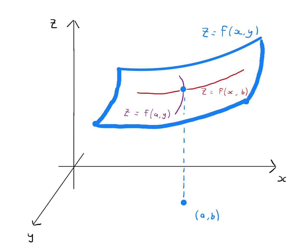
Suppose $(a,b)$ is a stationary point of a function $f(x,y)$. Graphically one can take two cross-sections of the surface $z=f(x,y)$ through the planes $x=a$ and $y=b$ respectively. This will describes two curves, one given in the $(y,z)$-plane by the univariate function $z=f(a,y)$, and the other given in the $(x,z)$-plane by the univariate function $z=f(x,b)$.These curves will have stationary points, in the context of univariate functions, at $y=b$ and $x=a$ respectively.

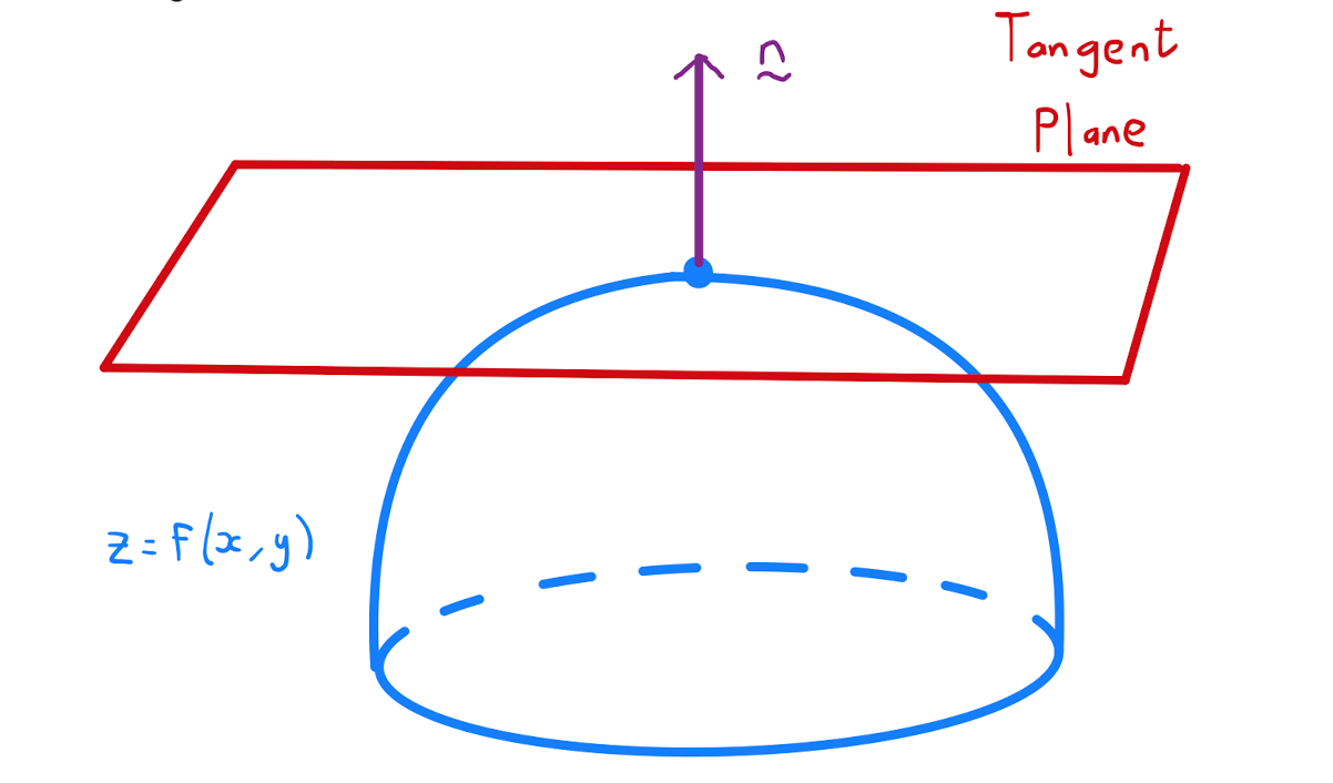
Describing the surface of $f$ using an implicit function, namely $F(x,y,z) = z - f(x,y)=0$, allows us to calculate a normal vector as per Section 7.1. Specifically a normal is given by $$\begin{align*} \nabla F &= \left( \frac{\partial F}{\partial x}, \frac{\partial F}{\partial y}, \frac{\partial F}{\partial z} \right) \\ &= \left( -f_x, -f_y, 1 \right) \\ &= (0,0,1). \end{align*}$$

It follows that the tangent plane to $z=f(x,y)$ is horizontal at a stationary point.

Definition 9.1.1 generalises to any multivariate function.

A stationary point of $f(x_1, x_2, \ldots , x_n)$ is a point such that $f_{x_i} =0$, for all $i = 1,2,\ldots n$.

There are three types of stationary points:

• Local maximum;

• Local minimum;

• Saddle point.

We will study each of these in turn in the following sections.

9.2 Local Maxima and Minima

Let $(a,b)$ be a stationary point of a function of two variables $f(x,y)$.

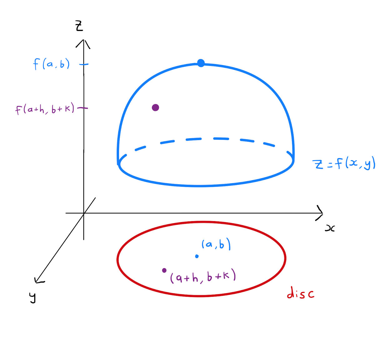
The value $f(a,b)$ of $f$ at $(a,b)$ is a local maximum if

$$f(a,b) \geq f(x,y), \qquad \text{for all } (x,y) \text{ in } D,$$

where $D$ is some open disc with center $(a,b)$.

The value $f(a,b)$ of $f$ at $(a,b)$ is a local minimum if

$$f(a,b) \leq f(x,y), \qquad \text{for all } (x,y) \text{ in } D,$$

where $D$ is some open disc with center $(a,b)$.

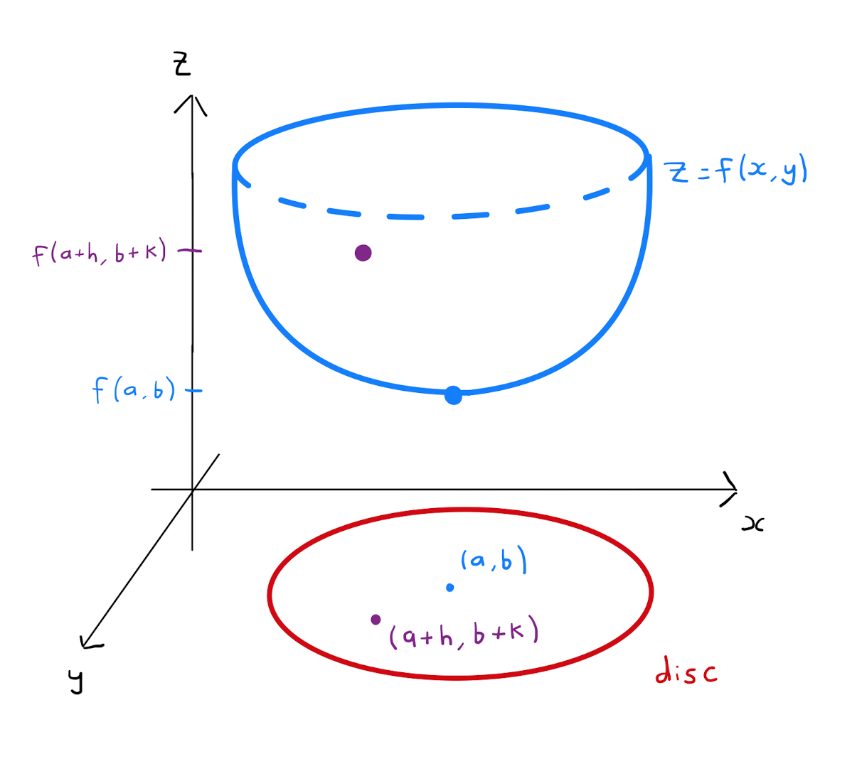
Any size of the disc $D$ in Definition 8.2.1 and Definition 8.2.2 will do, no matter how small. It is also worth noting the terminology local: there may be other points at which the function is smaller than a local minimum or greater than a local maximum, but these will be a distance away from the stationary point.

Consider the function $f(x,y) = x^2 + y^2$ from Example 9.1.2. We know there is a unique stationary point at $(0,0)$. Calculate that

$$\begin{align*} &f(0,0) = 0, \\ &f(x,y) = x^2 + y^2 > 0, \qquad \text{for } (x,y) \neq (0,0). \end{align*}$$

Therefore $(0,0)$ is a minimum stationary point.

9.3 Saddle Points

Let $(a,b)$ be a stationary point of a function of two variables $f(x,y)$.

The point $(a,b)$ is a saddle point of $f$ if for every disc $D$ with center $(a,b)$ there exists

• a point $(x_1,y_1) \in D$ such that $f(x_1,y_1) > f(a,b)$;

• a point $(x_2,y_2) \in D$ such that $f(x_2,y_2) < f(a,b)$.

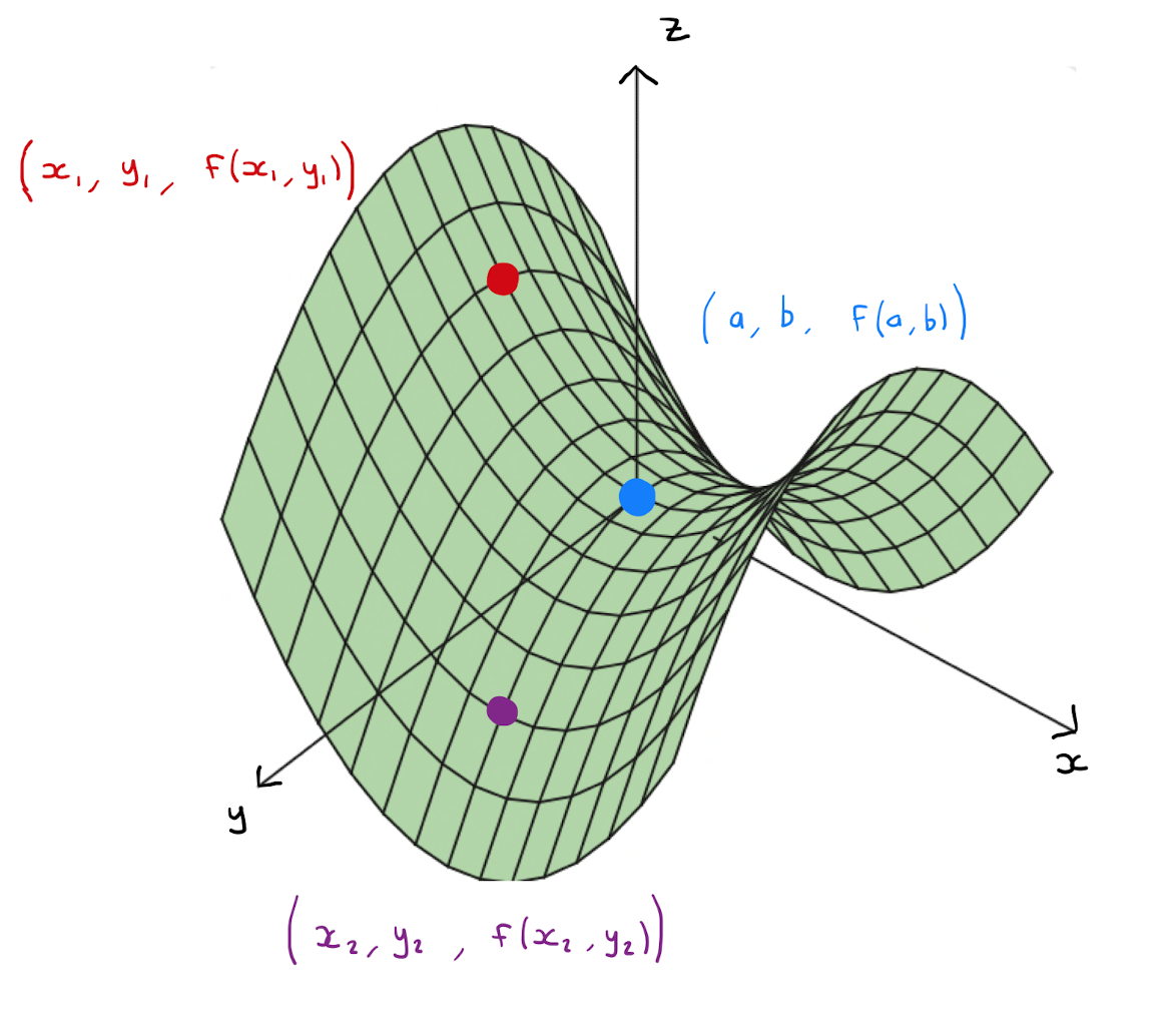
Equivalently a saddle point is a stationary point that is neither a local maximum or a local minimum.

9.4 Classification of Stationary Points

Suppose $f(x,y)$ has a stationary point at $(a,b)$. How can one tell if this stationary point is a local maximum, a local minimum or a saddle point?

Let $f$ be a function with continuous second order partial derivatives. The Hessian of $f$ is $$H(x,y) = f_{xx} f_{yy} - f_{xy}^{2}$$

Let $f$ be a function with a stationary point at $(a,b)$, and continuous second order partial derivatives in a disc centered at $(a,b)$. Then

• If $H(a,b)< 0$, then $f$ has a saddle point at $(a,b)$;

• If $H(a,b) >0$ and $f_{xx}(a,b)>0$, then $f$ has a local minimum at $(a,b)$;

• If $H(a,b) >0$ and $f_{xx}(a,b)<0$, then $f$ has a local maximum at $(a,b)$;

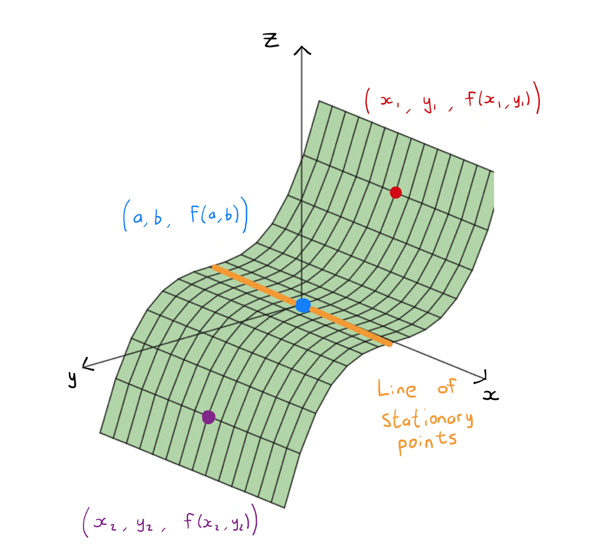
• If $H(a,b) = 0$, then no conclusion can be made about the classification of $(a,b)$.

Let $h,k$ be suitably small variables so that $(a+h,b+k)$ is contained in the disc centered at $(a,b)$ in which $f$ has continuous second order partial derivatives

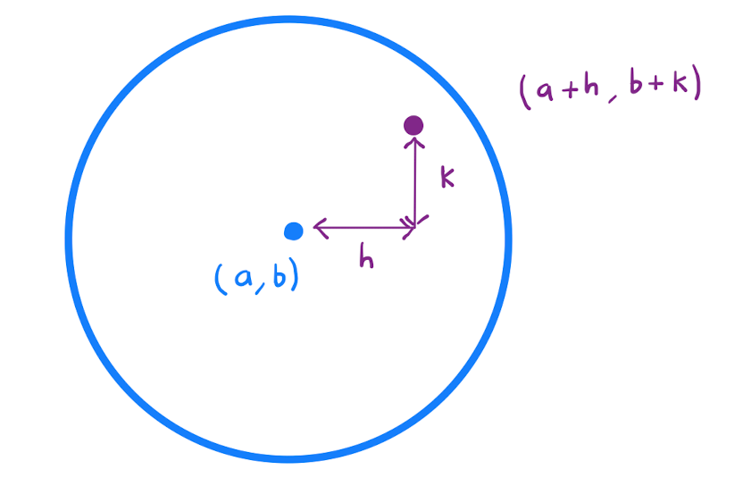
By Taylor’s theorem with $n=1$, one has $$f(a+h,b+k) = f(a,b) + h f_x (a,b) + k f_y (a,b) + R_1,$$ where $$R_1 = \frac{1}{2} \bigg( h^2 f_{xx}(a+th,b+tk) + 2hk f_{xy}(a+th,b+tk) + k^2 f_{yy}(a+th,b+tk) \bigg),$$ for some $t \in [0,1]$. Substituting in that $f_{x}(a,b) = f_{y}(a,b)=0$ and rearranging, one obtains $$f(a+h,b+k) - f(a,b) = R_{1}.$$ Hence the sign of $R_1$ is key to the classification of the stationary point $(a,b)$ since it determines whether $f$ increases or decreases away from $f$. Specifically for a fixed value of $h,k$:

• $R_1 \left( \frac{h}{k} \right) >0, \quad \implies \quad f(a+h,b+k) > f(a,b)$;

• $R_1 \left( \frac{h}{k} \right) <0, \quad \implies \quad f(a+h,b+k) < f(a,b)$.

Rearranging:

$$\begin{align*} R_1 &= \frac{1}{2} \bigg( h^2 f_{xx} + 2hk f_{xy} + k^2 f_{yy} \bigg) \\ &= \frac{k^2}{2} \bigg( f_{xx} \left(\frac{h}{k}\right)^2 + 2f_{xy} \frac{h}{k} + f_{yy} \bigg). \end{align*}$$

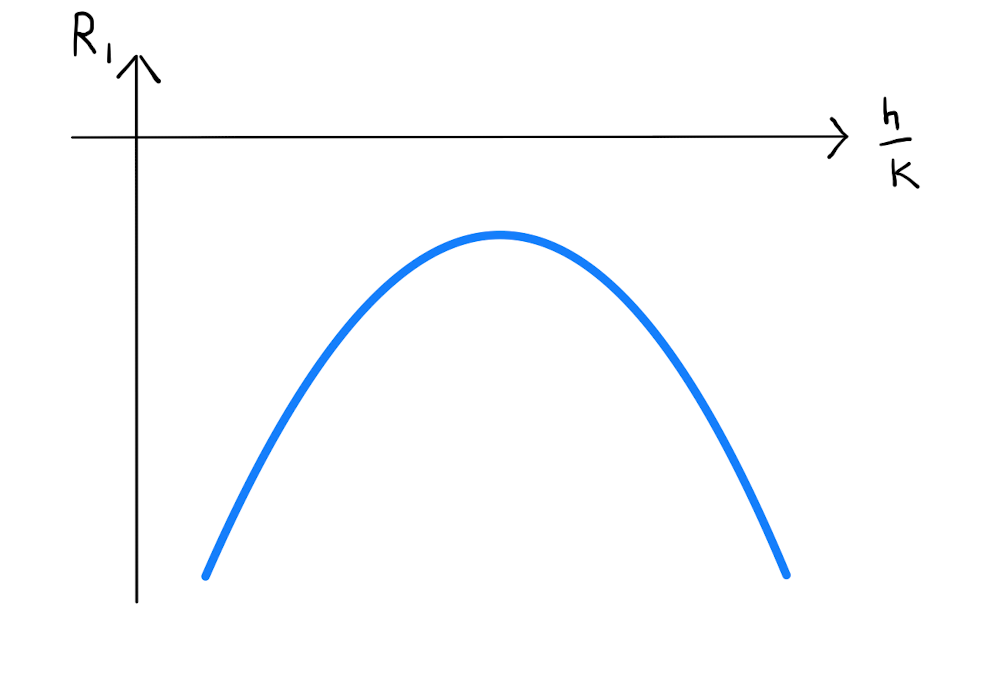
So $R_1$ can be thought of a quadratic function in the single variable $\frac{h}{k}$. Since we are only interested in the sign of $R_1$, and $\frac{k^2}{2}$ is always positive, it is enough to consider the quadratic function $$\widetilde{R_1} \left( \frac{h}{k} \right) = f_{xx} \left(\frac{h}{k}\right)^2 + 2f_{xy} \frac{h}{k} + f_{yy}$$ Quadratic functions are well-understood. In particular for a general quadratic $Q(x) = ax^2 + bx + c$, the roots of $Q$ are governed by the discriminant $\Delta_Q = b^2 -4ac$. With this in mind, define: $$\begin{align*} \Delta &= \Delta_{\widetilde{R_1} \left(\frac{h}{k}\right)} \\ &= \left( 2 f_{xy} \right)^2 - 4 f_{xx} f_{yy} \\ &= 4 \left( f_{xy}^{2} - f_{xx}f_{yy} \right). \end{align*}$$

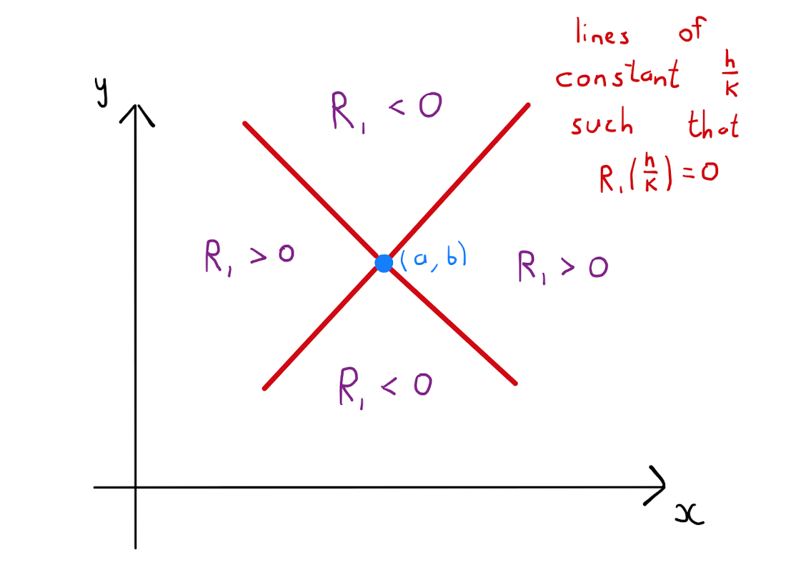
Suppose that $\Delta>0$. Then $\widetilde{R_1}$ has two real roots.

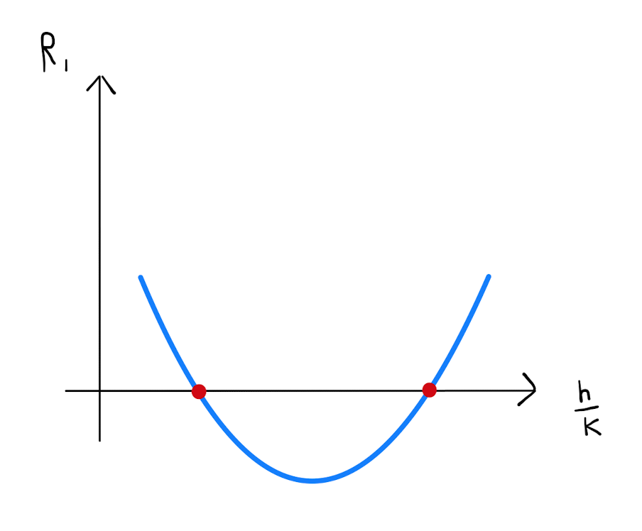
Specifically there are two distinct values for $\frac{h}{k}$ for which $R_1=0$. At both of these roots $R_1$ changes sign, and $(a,b)$ is therefore a saddle point.

Alternatively suppose $\Delta <0$, that is that $\widetilde{R_1}$ has no real roots. Then $R_1$ will always have the same sign, be that positive or negative. Therefore $(a,b)$ is either a local minimum or a local maximum.

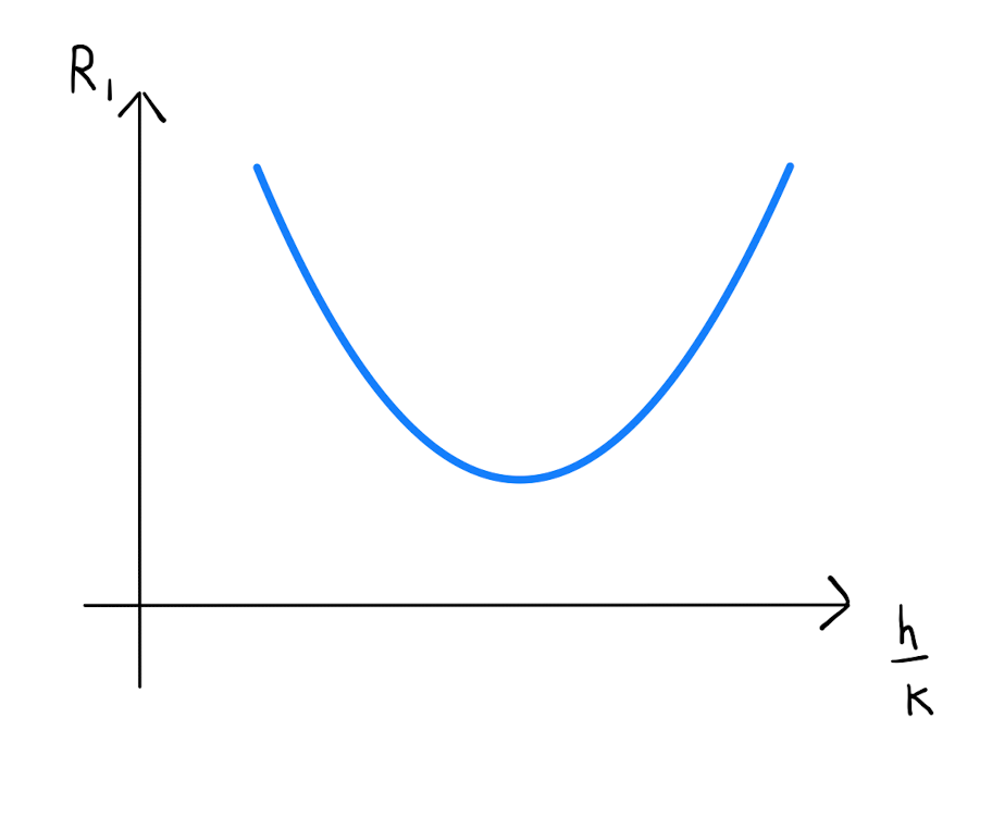
Since in this case the sign of $R_{1}$ does not change, it can be found by looking at a single point. Specifically when $k=0$, we have $R_{1} = \frac{h^2}{2} f_{xx}$. Hence

• $f_{xx} >0 \quad \implies \quad R_{1} > 0 \quad \implies \quad (a,b)$ is a local minimum;

• $f_{xx} <0 \quad \implies \quad R_{1} < 0 \quad \implies \quad (a,b)$ is a local maximum.

Noting that $\Delta = -4 H$ gives the desired result.

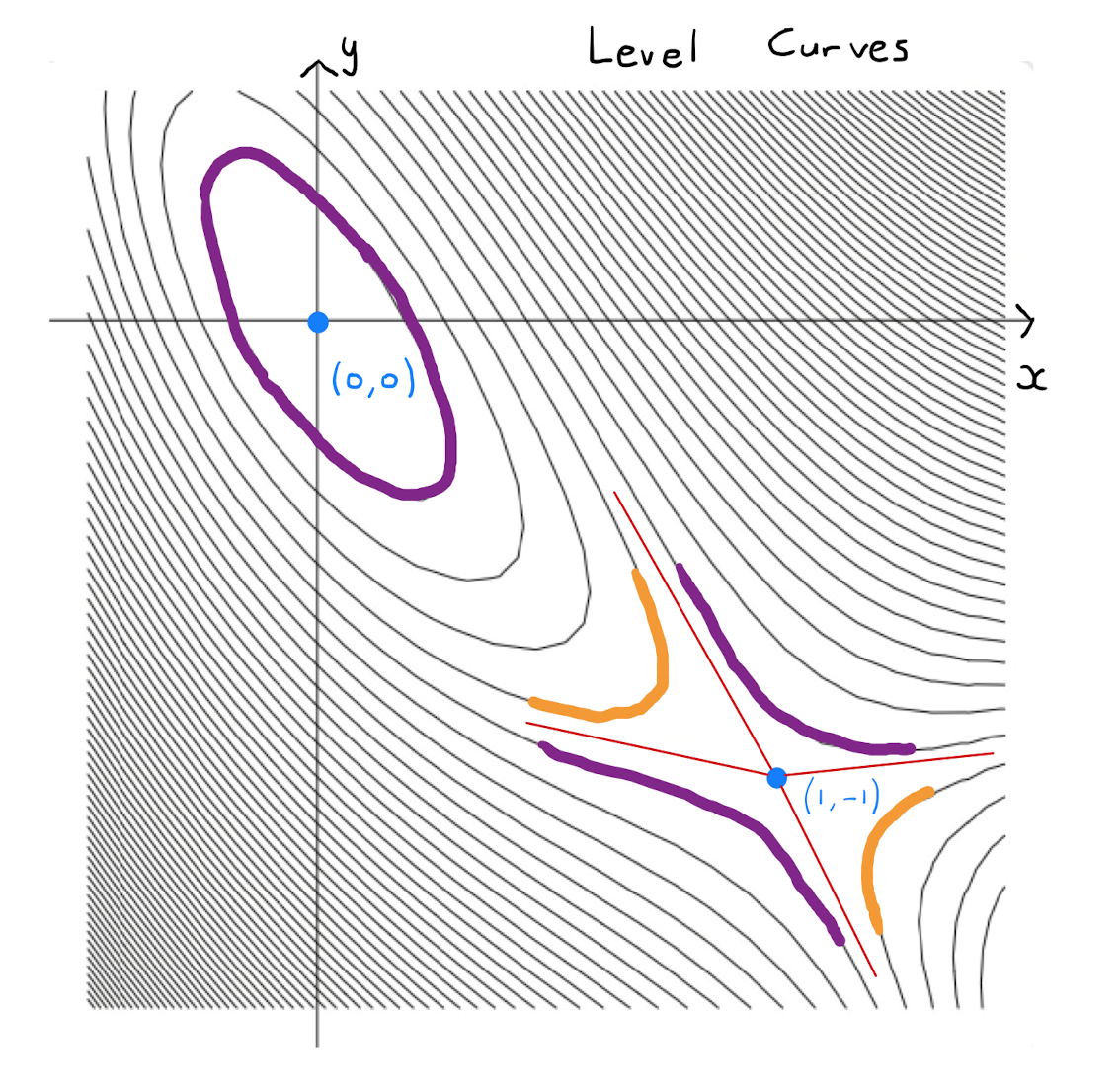
Find and classify the stationary points of $$f(x,y) = 6x^2 - 2 x^3 + 3y^2 + 6xy.$$
Equating the two first order partial derivatives of $f$ to zero, one obtains $$\begin{align*} f_x &= 12x -6x^2 + 6y = 0 \tag{$\star$}, \\ f_y &= 6y + 6x = 0 \tag{$\star \star$}. \end{align*}$$

Substituting $(\star \star)$ into $(\star)$ gives

$$\begin{align*} 12x - 6 x^2 - 6x &= 0, \\ x(1-x) &= 0, \\ \implies \quad x=0 \text{ or } x&=1. \end{align*}$$

When $x=0$, equation $(\star \star)$ dictates $y=0$, and when $x=1$, equation $(\star)$ dictates $y=-1$. Therefore $f$ has two stationary points: $(0,0)$ and $(1,-1)$.

Calculating the second order partial derivatives of $f$, one obtains:

$$\begin{align*} f_{xx} &= 12 -12x, \\ f_{xy} &= 6, \\ f_{yy} &= 6. \end{align*}$$

The Hessian of $f$ is then given by

$$H(x,y) = f_{xx} f_{yy} - f_{xy}^{2} = 6(12-12x) - 36= 36 - 72x.$$

By Theorem 9.4.2, the stationary points are classified as follows:

• $H(0,0) =36>0$ and $f_{xx} =12 >0, \quad \implies \quad$ the stationary point $(0,0)$ is a local minimum;

• $H(1,-1) =-36<0, \quad \implies \quad$ the stationary point $(1,-1)$ is a saddle point.