Chapter 5 Small changes and Differentials

5.1 Small Changes

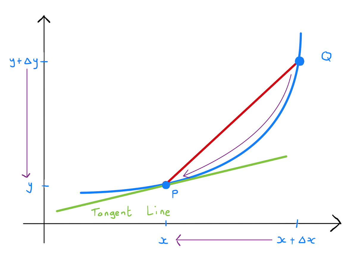
Consider a univariate function \(y=y(x)\). Suppose that the variable \(x\) from a fixed value undergoes some small increase \(\Delta x\). Subsequently, as the dependent variable, there will be some small change in \(y\), denoted \(\Delta y\). One asks how the change \(\Delta y\) can be expressed in terms of \(\Delta x\).

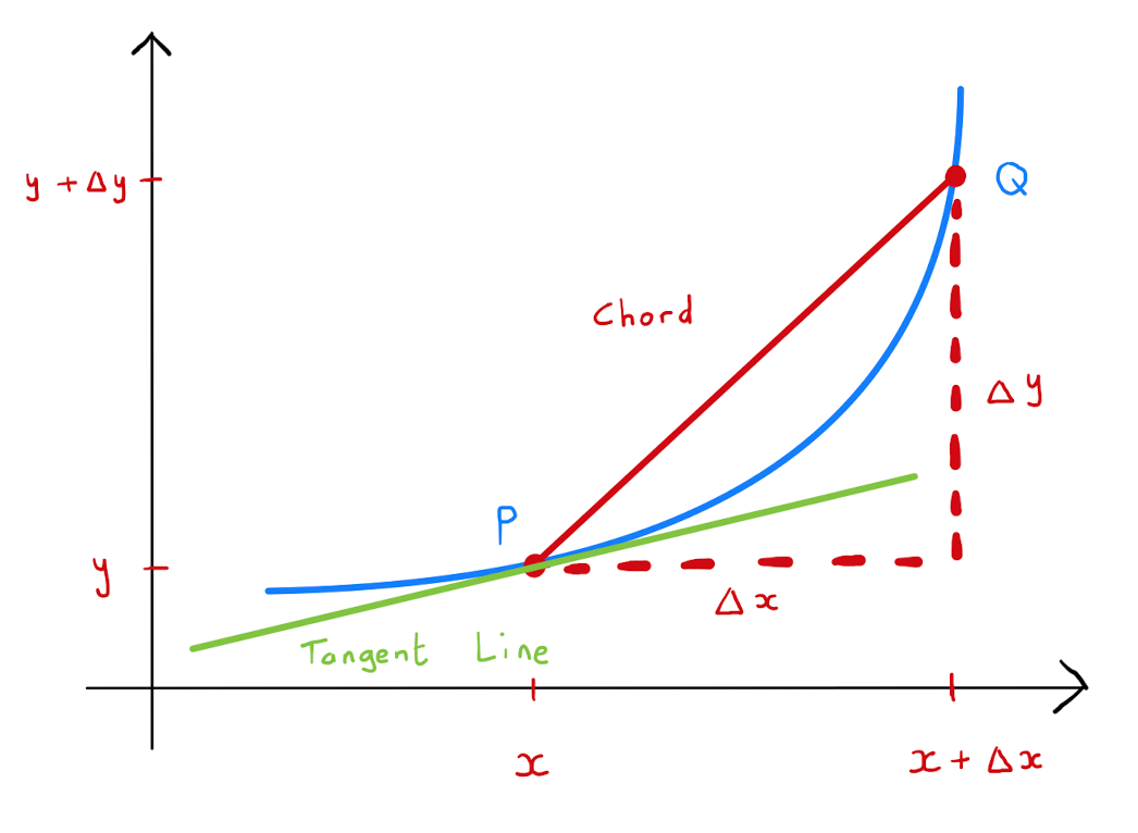
The ratio of \(\Delta y\) to \(\Delta x\) is equal to the gradient of the chord between the points \(P=(x,y)\) and \(Q=(x+\Delta x, y+ \Delta y)\). Provided that \(\Delta x\) is sufficiently small, this chord is ‘close’ to lying on the tangent line at \(P\). Specifically the gradient of the chord \(PQ\) can be approximated by the gradient of the tangent line, which is \(\frac{d y}{dx}\). Written mathematically: \[\begin{align*} \frac{\Delta y}{\Delta x} &= \text{gradient of chord } PQ \\ &\approx \text{gradient of tangent line at } P \\ &= \frac{dy}{dx} \end{align*}\] Rearranging one concludes that the small changes \(\Delta x\) and \(\Delta y\) are related by \[\Delta y \approx \frac{dy}{dx} \Delta x.\]

How is this analysis replicated in the case of an implicit function of two variables \(z=z(x,y)\)? Well \(\Delta z\) will be given by the difference between \(z(x,y)\) and \(z(x+\Delta x, y+ \Delta y)\). To investigate this quantity consider the parallogram on the surface \(z = z(x,y)\) whose vertices are given by the points above \((x,y),(x+\Delta x, y),(x, y+ \Delta y)\) and \((x+\Delta x, y+ \Delta y)\).

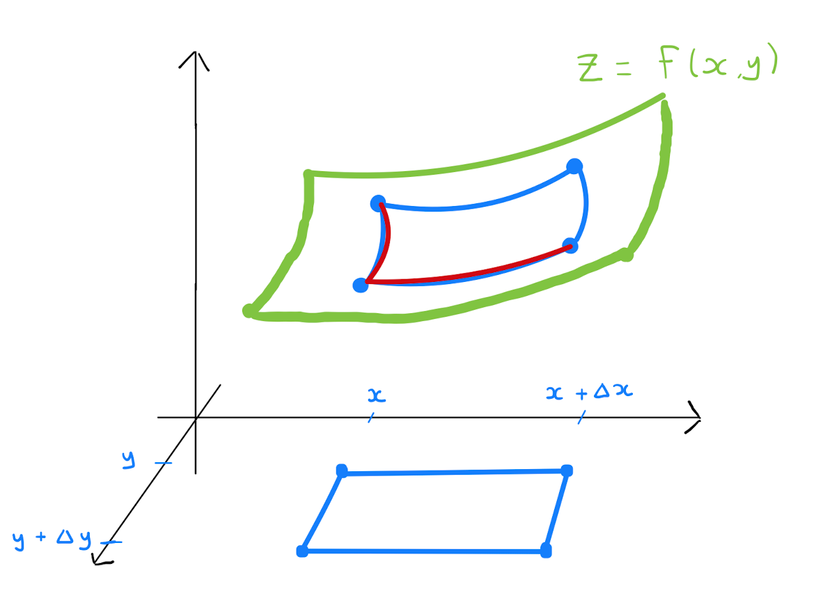
Decomposing the expression for \(\Delta z\): \[\begin{align*} \Delta z &= z(x+\Delta x, y+ \Delta y) - z(x,y) \\ &= \Big( z(x+\Delta x, y+ \Delta y) - z(x+\Delta x, y) \Big) + \Big( z(x+\Delta x, y) - z(x, y) \Big). \end{align*}\] Each bracket represents a change in the dependent variable \(z\) as only one of the independent variables is allowed to vary. When studying the term \(z(x+\Delta x, y) - z(x, y)\), one can treat the \(y\) variable as a fixed constant, and treat \(z\) as a function in the single variable \(x\).

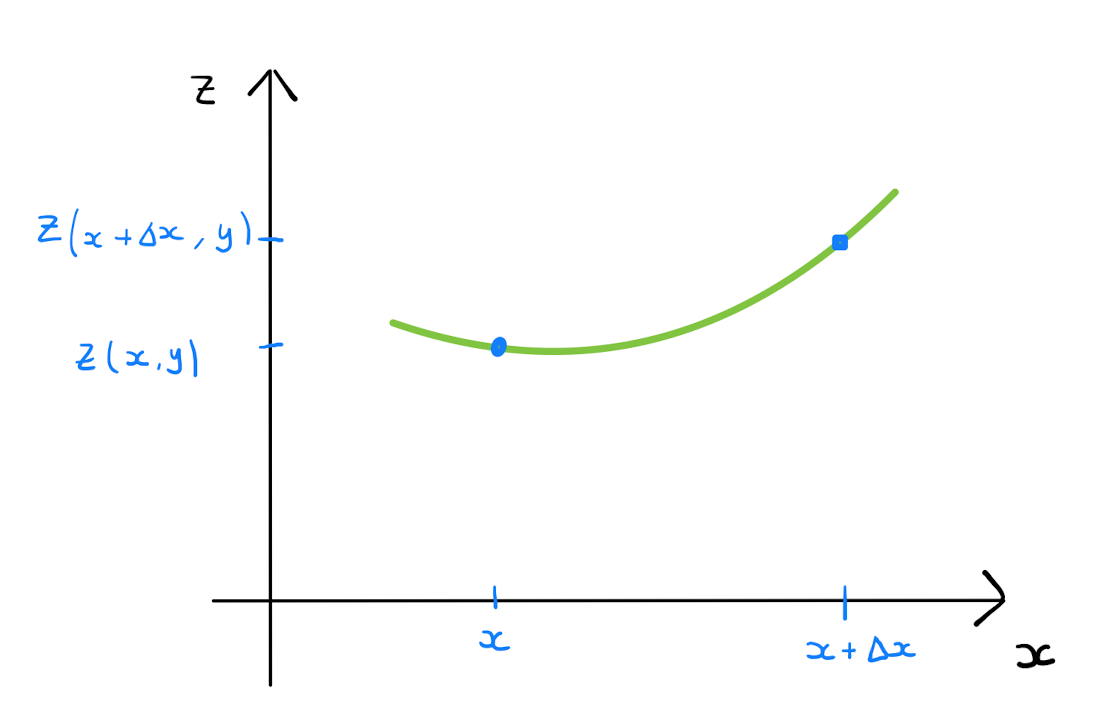
Applying the theory of small changes for univariate functions here gives \[z(x+\Delta x, y) - z(x, y) \approx \Delta x \frac{\partial z}{\partial x}.\]

Similarly the expression \(z(x+\Delta x, y+ \Delta y) - z(x+\Delta x, y)\) lends itself to thinking of \(z\) as a univariate function. However before doing so, note that since \(\Delta x\) is sufficiently small, one can approximate the difference \(z(x+\Delta x, y+ \Delta y) - z(x+\Delta x, y)\) by \(z(x, y+ \Delta y) - z(x, y)\).

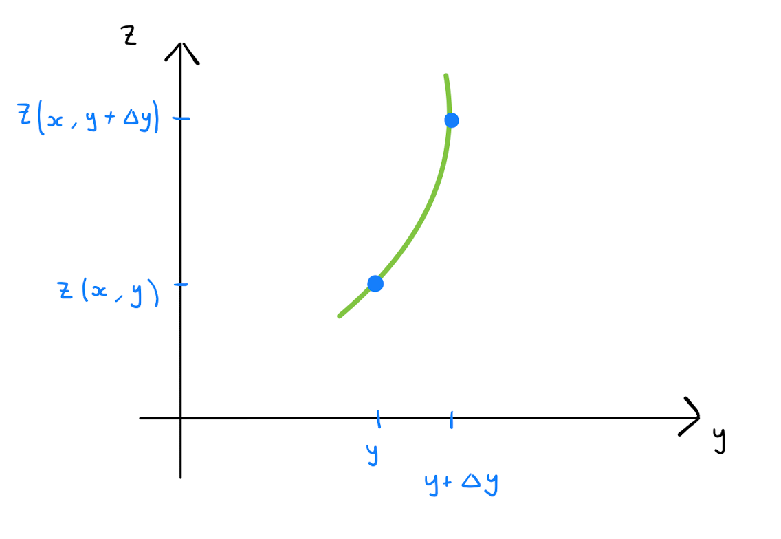
By treating \(x\) as a fixed value and \(y\) as the sole variable, one concludes by the theory of small changes for univariate functions that \[z(x+\Delta x, y+ \Delta y) - z(x+\Delta x, y) \approx \Delta y \frac{\partial z}{\partial y}\]

Therefore one can approximate \(\Delta z\) by \[\Delta z \approx \frac{\partial z}{\partial x} \Delta x + \frac{\partial z}{\partial y} \Delta y.\]

The volume \(V\) of a cylinder is given in terms of the radius \(r\) and height \(h\) by the formula \(V= \pi r^2 h\). Find \(\Delta V\) in terms of small changes \(\Delta r\) and \(\Delta h\), both by direct compution and by using the theory of small changes.

‘Direct Computation’ \[\begin{align*} V + \Delta V &= \pi (r + \Delta r)^2 (h + \Delta h) \\ &= \pi (r^2 + 2 r \Delta r + \Delta r^2)(h + \Delta h) \\ &= \pi r^2 h + 2 \pi rh \Delta r + \pi h \Delta r^2 + \pi r^2 \Delta h + 2 \pi r \Delta r \Delta h + \pi \Delta r^2 \Delta h \\ &= \left( \pi r^2 h \right) + \left( 2 \pi rh \Delta r + \pi r^2 \Delta h \right) + \text{'higher order terms in $\Delta r$ and $\Delta h$'} \\ &\approx V + 2 \pi rh \Delta r + \pi r^2 \Delta h, \\ \Delta V &\approx 2 \pi rh \Delta r + \pi r^2 \Delta h. \end{align*}\]

‘Theory of Small Changes’
Since \(V = \pi r^2 h\), calculate:

\[\begin{align*} \frac{\partial V}{\partial r} &= 2 \pi r h, \\[5pt] \frac{\partial V}{\partial h} &= \pi r^2. \end{align*}\]

It follows

\[\begin{align*} \Delta V &\approx \frac{\partial V}{\partial r} \Delta r + \frac{\partial V}{\partial h} \Delta h \\ &= 2 \pi r h \Delta r + \pi r^2 \Delta h. \end{align*}\]

Note the comparative ease of using the theory of small changes compared to the direct computation, even with a relatively straightforward function.

Considering again the cylinder of Example 5.1.1, if the radius \(r\) and height \(h\) increase by \(3 \%\) and \(1 \%\) respectively what is the approximate percentage increase in the volume \(V\)?

The percentage increase of \(r\) and \(h\) tell us that

\[\frac{\Delta r}{r} = 0.03, \qquad \text{and} \qquad \frac{\Delta h}{h} = 0.01.\] Using the Example 5.1.1, the proportion by which \(V\) increases is given by \[\begin{align*} \frac{\Delta V}{V} &= \frac{2 \pi r h \Delta r + \pi r^2 \Delta h}{\pi r^2 h} \\ &= 2 \frac{\Delta r}{r} + \frac{\Delta h}{h} \\ &= 2 \cdot 0.03 + 0.01 \\ &= 0.07 \end{align*}\]

Therefore \(V\) will increase by \(7 \%\).

5.2 Differentials

Looking again at the univariate function \(y=y(x)\) consider the limit in the theory of Section 5.1 as \(\Delta x \rightarrow 0\), that is as the change made in \(x\) becomes infintesimally small. The approximation \(\Delta y \approx \frac{d y}{d x} \Delta x\) becomes an equality and is written in the form \[dy = \frac{dy}{dx} dx.\]

The infinitesimal changes \(dx\) and \(dy\) are called differentials.

Similarly looking at a function of two variables \(z=z(x,y)\), and considering small changes \(\Delta x, \Delta y\) in the variables \(x\) and \(y\) respectively. The corresponding change in \(z\) is given approximately by \(\Delta z \approx \frac{\partial z}{\partial x} \Delta x + \frac{\partial z}{\partial y} \Delta y\). Letting both \(\Delta x, \Delta y \rightarrow 0\), that is letting both changes become infinitesimally small, the approximation becomes an equality of differentials: \[dz = \frac{\partial z}{\partial x} dx + \frac{\partial z}{\partial y} dy.\] The differentials \(dx\) and \(dy\) are treated as independent variables.

Let \(x=x(r,\theta) = r \cos \theta\) and \(y= y(r,\theta) = r \sin \theta\). Use differentials to find \(\frac{\partial r}{\partial x}\) and \(\frac{\partial r}{\partial y}\).

Note that one cannot assume \(\frac{\partial r}{\partial x} \neq \frac{1}{\left( \frac{\partial x}{\partial r} \right)}\) as is the case for multivariate functions in general. This is a key difference between the ordinary derivative of a univariate function and partial derivatives.

Instead apply the theory of differentials to obtain \[\begin{equation*}\tag{$\star$} dx = \frac{\partial x}{\partial r} dr + \frac{\partial x}{\partial \theta} d \theta = \cos \theta dr + (-r \sin \theta) d\theta, \end{equation*}\] and \[\begin{equation}\tag{$\star \star$} dy = \frac{\partial y}{\partial r} dr + \frac{\partial y}{\partial \theta} d \theta = \sin \theta dr + r \cos \theta d\theta. \end{equation}\] Calculating \(\cos \theta \cdot (\star) + \sin \theta \cdot (\star \star)\), obtain \[\begin{align*} \cos \theta \cdot dx + \sin \theta \cdot dy &= \cos^{2} \theta \cdot dr - r \sin \theta \cos \theta \cdot d \theta + \sin^{2} \theta \cdot dr + r \sin \theta \cos \theta \cdot d\theta \\ &= \left( \cos^{2} \theta + \sin^{2} \theta \right) dr \\ &= dr. \end{align*}\] Alternatively the variable \(r\) could be thought of in terms of \(x\) and \(y\). Therefore by the theory of differentials \(dr = \frac{\partial r}{\partial x} dx + \frac{\partial r}{\partial y} dy\). By comparing coefficients of \(dx\) and \(dy\) between the two obtained expressions for \(dr\), one obtains \[ \frac{\partial r}{\partial x} = \cos \theta, \qquad \text{and} \qquad \frac{\partial r}{\partial y} = \sin \theta.\]

Calculate \(\frac{\partial \theta}{\partial x}\) and \(\frac{\partial \theta}{\partial y}\) from Example 5.2.2 using the theory of differentials.