Chapter 10 Lagrange Multipliers

10.1 Extreme Values with a Constraint

The study of stationary points provides us with a method by which to calculate local maximums and minimums of multivariate functions. In this chapter we ask a more general question: how can one find the extremal values (maximums and minimums) of a function $f$ subject to a constraint $g=0$. That is, $f$ is only evaluated at points where $g$ evaluates to $0$? Initially consider the case where $f(x,y)$ and $g(x,y)$ are functions of two variables.

Sometimes such a problem can be tackled directly.

Find the minimum value of $f(x,y)=4x^2 +3y^2$ subject to the constraint $g(x,y)=y+2x-8=0$.

Manipulating $g(x,y)=0$ to obtain an expression for $y$:

\[\begin{align*} y+2x-8 &= 0, \\ y &= 8-2x. \end{align*}\]

Eliminating $y$ from the expression for $f$ obtain

\[\begin{align*} F(x) &= f(x,8-2x), \\ &= 4x^2 + 3(8-2x)^2, \\ &= 16x^2 -96x + 192. \end{align*}\]

$F$ is a univariate function, and a minimum turning point of $F$ will lead to a solution to the constraint problem. Calculating the derivatives of $F$:

\[\begin{align*} \frac{dF}{dx} &= 32x -96, \\[3pt] \frac{d^2 F}{dx^2} &= 32. \\ \end{align*}\]

Solving $\frac{dF}{dx} = 32x -96=0$ gives $x=3$. Since $\frac{d^2 F}{dx^2}(3) = 32 >0$, this turning point is a minimum. At $x=3$, calculate

\[y= 8-2 \cdot 3=2,\]

and

\[f(3,2)= 4\cdot 3^2 +3 \cdot 2^2 = 48.\]

Hence $4x^2 + 3y^2$ subject to the constraint $y+2x-8=0$ has minimum value 48 at the point $(3,2)$.

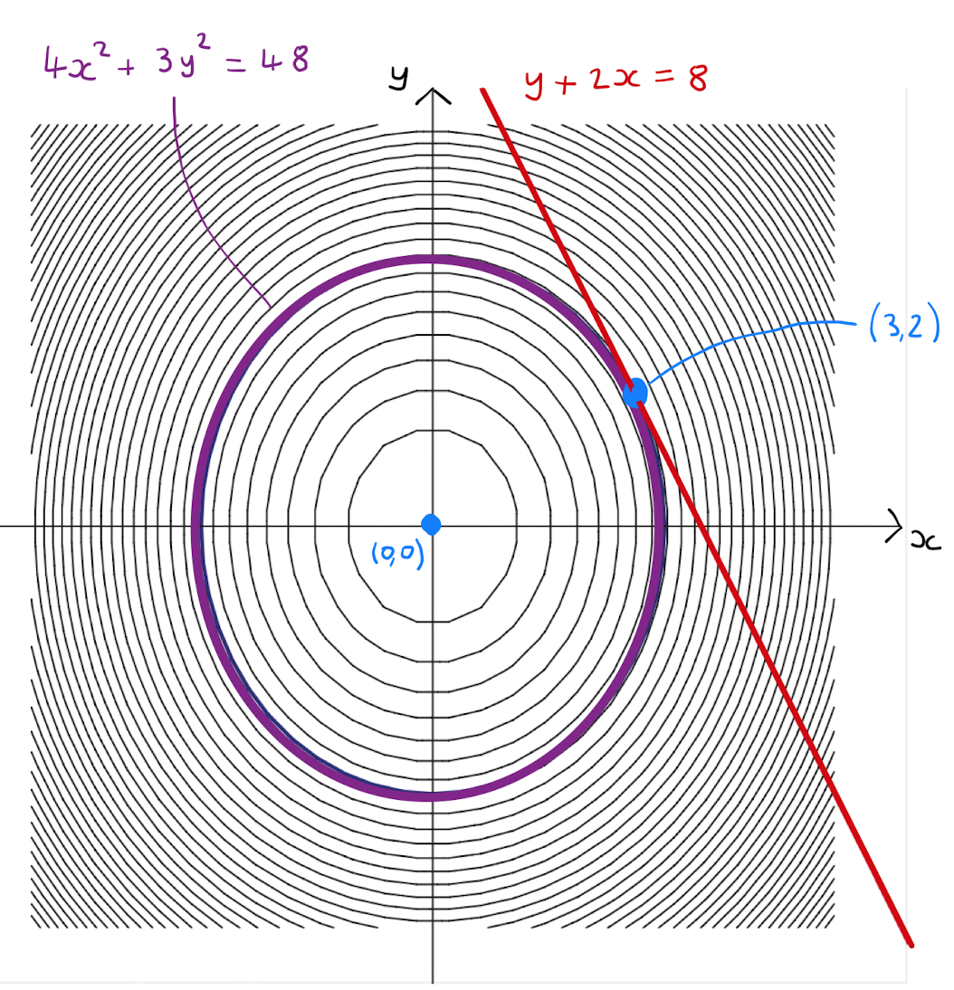
Example 10.1.1 has an interesting geometric interpretation. The constraint $g(x,y)=y+2x-8=0$ is the equation of a straight line in the $(x,y)$-plane. The level curves of $z=f(x,y)$ at height $\lambda \geq 0$ are ellipses $4x^2+3y^2 = \lambda$ with center $(0,0)$ in the $(x,y)$-plane. As $\lambda$ increases from $0$, the ellipse gets bigger until it touches the line $y+2x-8=0$. This point of contact occurs at the point $(3,2)$ between the line and the level curve at height $\lambda =48$. For any smaller value for $\lambda$, there is no contact and so the constraint is not satisfied for points on the level curve.

It is not hard to see that this direct computation method would fail for expressions of $f$ and $g$ that are more complicated, or in the case that $f$ and $g$ have more than two variables. We require a more general method to solve this constraint problem.

10.2 Method of Lagrange Multipliers

The technique used to solve these extrema values under a constraint problem is method of Lagrange multipliers.

Let $f(x,y)$ and $g(x,y)$ be functions of two variables. Let $\lambda$ be a new variable, and define

\[F(x,y,\lambda) = f(x,y) - \lambda g(x,y).\]

Then a stationary point $(x_0,y_0,\lambda_0)$ of $F(x,y,\lambda)$ corresponds to an extremal point $(x_0,y_0)$ of $f(x,y)$ subject to the constraint $g(x,y)=0$.

The variable $\lambda$ is called the Lagrange multiplier.

We solve the problem posed in Example 10.1.1 again, this time using the method of Lagrange multipliers instead of a direct computation.

Find the extrema values of $f(x,y)=4x^2 +3y^2$ subject to the constraint $g(x,y)=y+2x-8=0$.

By the method of Lagrange multipliers define

\[\begin{align*} F(x,y,\lambda) &= f(x,y) - \lambda g(x,y) \\ &= 4x^2 +3y^2 - \lambda ( y+2x-8 ). \end{align*}\]

To find the stationary points of $F$, equate the partial derivatives to $0$:

\[\begin{align*} F_{x} &= 8x-2\lambda =0 \tag{$\star$}\\ F_{y} &= 6y- \lambda=0 \tag{$\star \star$}\\ F_{\lambda} &= -y-2x+8=0 \tag{$\star \star \star$} \end{align*}\]

Solving these equations simultaneously:

\[\begin{align*} \frac{1}{2}(\star) - (\star \star): \qquad 4x - 6y &=0 \\ 2x &= 3y, \tag{$\dagger$} \\ \text{Sub } (\dagger) \text{ into } (\star \star \star): \qquad 4y-8 &= 0 \\ y &= 2, \\ (\dagger) \implies \qquad x &= 3, \\ (\star \star) \implies \qquad \lambda &= 12. \end{align*}\]

Therefore by the method of Lagrange multipliers, an extrema value is obtained at $(3,2)$ and this point calculate $f(3,2)=48$.

The solution to Example 10.2.1 was the same as that obtained by direct computation in Example 10.1.1.

One drawback of the method of Lagrange multipliers is that it doesn’t tell us whether the extrema is a maximum or minimum. In Example 10.2.1, one has that $4x^2 + 3y^2 \geq 0, \forall (x,y)$ and so necessarily the function must have a minimum value. Since there was a unique extrema value $(3,2)$, this must be the minimum value.

The method of Lagrange multipliers generalises to finding extremal values of a function of $n$ variables subject to $m$ constraints.

Let $f(x_1,\ldots, x_n), g_1(x_1,\ldots, x_n), \ldots, g_m (x_1,\ldots, x_n)$ be multivariate functions of $n$ variables. Let $\lambda_1, \ldots, \lambda_m$ be new variables, and define

\[\begin{align*} F(x_1,\ldots, x_n,\lambda_1, \ldots, \lambda_m ) &= f(x_1,\ldots, x_n) - \sum\limits_{i=1}^{m} \lambda_i g_i(x_1,\ldots, x_n) \\ &= f - \sum\limits_{i=1}^{m} \lambda_i g_i \end{align*}\]

Then a stationary point $\left( \bar{x}_1,\ldots, \bar{x}_n,\bar{\lambda}_1, \ldots, \bar{\lambda}_m \right)$ of $F(x_1,\ldots, x_n,\lambda_1, \ldots, \lambda_m)$ corresponds to an extremal point $(\bar{x}_1,\ldots, \bar{x}_n)$ of $f(x_1,\ldots, x_n)$ subject to the constraints $g_1(x_1,\ldots, x_n) = \ldots g_m(x_1,\ldots, x_n)=0$.

Find the point on the hyperbolic cylinder $x^2 - z^2=4$ which is nearest to the origin.

The problem is equivalent to minimising $f(x,y,z)= x^2 + y^2 + z^2$ subject to the constraint $g(x,y,z)=x^2 -z^2-4=0$. By the method of Lagrange multipliers define

\[\begin{align*} F(x,y,z,\lambda) &= f(x,y,z) - \lambda g(x,y,z) \\ &= x^2 + y^2 + z^2 - \lambda ( x^2 -z^2-4 ). \end{align*}\]

To find the stationary points of $F$, equate the partial derivatives to $0$:

\[\begin{align*} F_{x} &= 2x-2x\lambda = 2x(1-\lambda) = 0, \tag{$\star$}\\ F_{y} &= 2y =0, \tag{$\star \star$} \\ F_{z} &= 2z + 2z \lambda = 2z (1 + \lambda) =0, \tag{$\dagger$} \\ F_{\lambda} &= -x^2 +z^2+4=0. \tag{$\dagger \dagger$} \end{align*}\]

Solving these equations simultaneously:

\[\begin{align*} (\star \star) \implies \qquad y &= 0, \\ (\star) \implies \qquad x &= 0 \text{ or } \lambda =1 \end{align*}\]

But if $x=0$, then $(\dagger \dagger)$ cannot have a real solution. Therefore

\[\begin{align*} y &=0 \text{ and } \lambda=1, \\ (\dagger) \implies \qquad z&=0, \\ (\dagger \dagger) \implies \qquad x^2 &= 4, \\ x &= \pm 2. \end{align*}\]

Therefore by the method of Lagrange multipliers, an extrema value is obtained at both $(2,0,0)$ and $(-2,0,0)$. Both points are a distance $2$ from the origin. Geometrically a minimum value of the distance must exist, and hence must be $2$.