Chapter 11 Double Integrals
11.1 Recap of Single Integrals
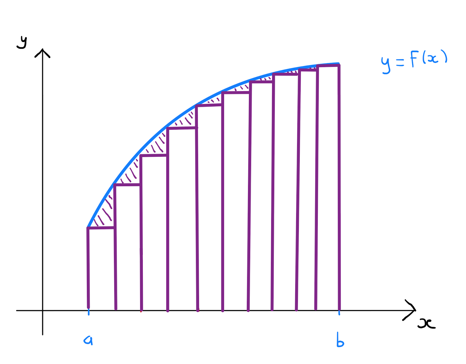
Consider a function \(y=f(x)\) and an interval \([a,b] \subset \mathbb{R}\). How is the integral of \(f(x)\) over the interval \([a,b]\), denoted \(\int_{a}^{b} f(x) \,dx\), defined formally?

First let \(\Delta x \geq 0\) be a sufficiently small real value such that \(n= \frac{b-a}{\Delta x} \in \mathbb{Z}\). Divide the interval \([a,b]\) into \(n\) sub-intervals. Specifically these sub-intervals are of the form:

For each of these sub-intervals form the product \(f(a+i\Delta x) \cdot \Delta x\). This expression is the area of a rectangle that approximates the area under the curve \(y=f(x)\) over the sub-interval \([a + i \Delta x, a+ (i+1)\Delta x]\).

By summing over all sub-intervals, that is \(\sum\limits_{i=0}^{\frac{b-a}{\Delta x}-1} f(a+i\Delta x) \cdot \Delta x\), one obtains an approximation of the area under the curve \(y=f(x)\) over the entirety of the interval \([a,b]\).

The idea is that in general, though not necessarily, smaller values of \(\Delta x\) will improve the approximation of the area.
Let \(\Delta x\) tend towards \(0\). If \(\sum\limits_{i=0}^{\frac{b-a}{\Delta x}-1} f(a+i\Delta x) \cdot \Delta x\) tends to a finite limit, then this value is the integral \(\int_{a}^{b} f(x) \,dx\) of \(f(x)\) over the interval \([a,b]\). Specifically
11.2 Definition of a Double Integral
Consider a function of two variables \(f(x,y)\), and a two-dimensional region \(R \subset \mathbb{R}^{2}\). The integral of \(f\) over \(R\), known as a double integral is defined in a similar fashion to a single integral.
Let \(\Delta x\) and \(\Delta y\) be two sufficiently small real values. Consider a rectangle in the \((x,y)\)-plane with a side of length \(\Delta x\) parallel to the \(x\)-axis, and a side of length \(\Delta y\) parallel to the \(y\)-axis. Fill \(R\) as much as possible with such rectangles. Note \(R\) may have curved boundaries, and so this packing process would not cover \(R\) exactly.
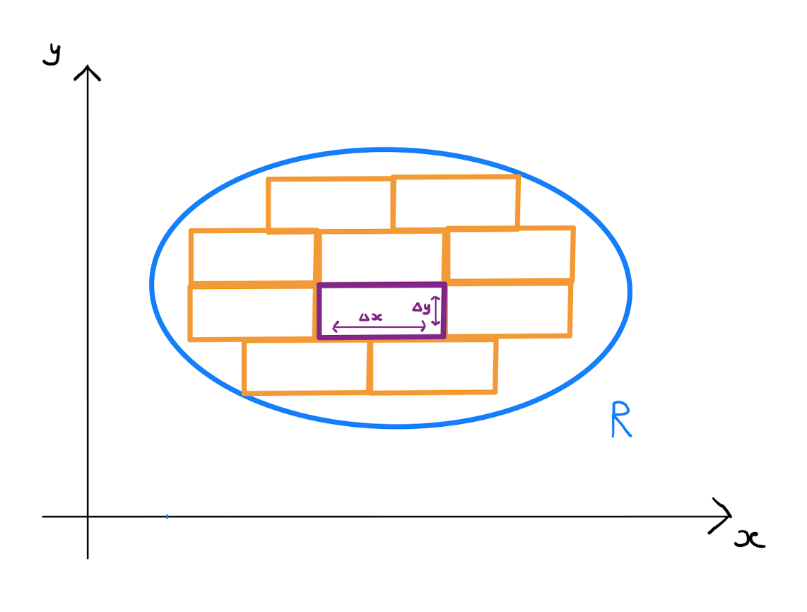
Enumerate the rectangles with labels \(R_1, \ldots R_n\). Rectangle \(R_i\) will have vertices \(\left( x_i, y_i \right)\), \(\left( x_i + \Delta x, y_i \right)\), \(\left( x_i, y_i + \Delta y \right)\) and \(\left( x_i + \Delta x, y_i + \Delta y \right)\) for some \(x_i,y_i \in \mathbb{R}\). For the rectangle \(R_i\) form the product \(f(x_i, y_i) \cdot \Delta x \Delta y\). This expression is the area of a cuboid that approximates the volume under the surface \(z=f(x,y)\) over the rectangle \(R_i\).
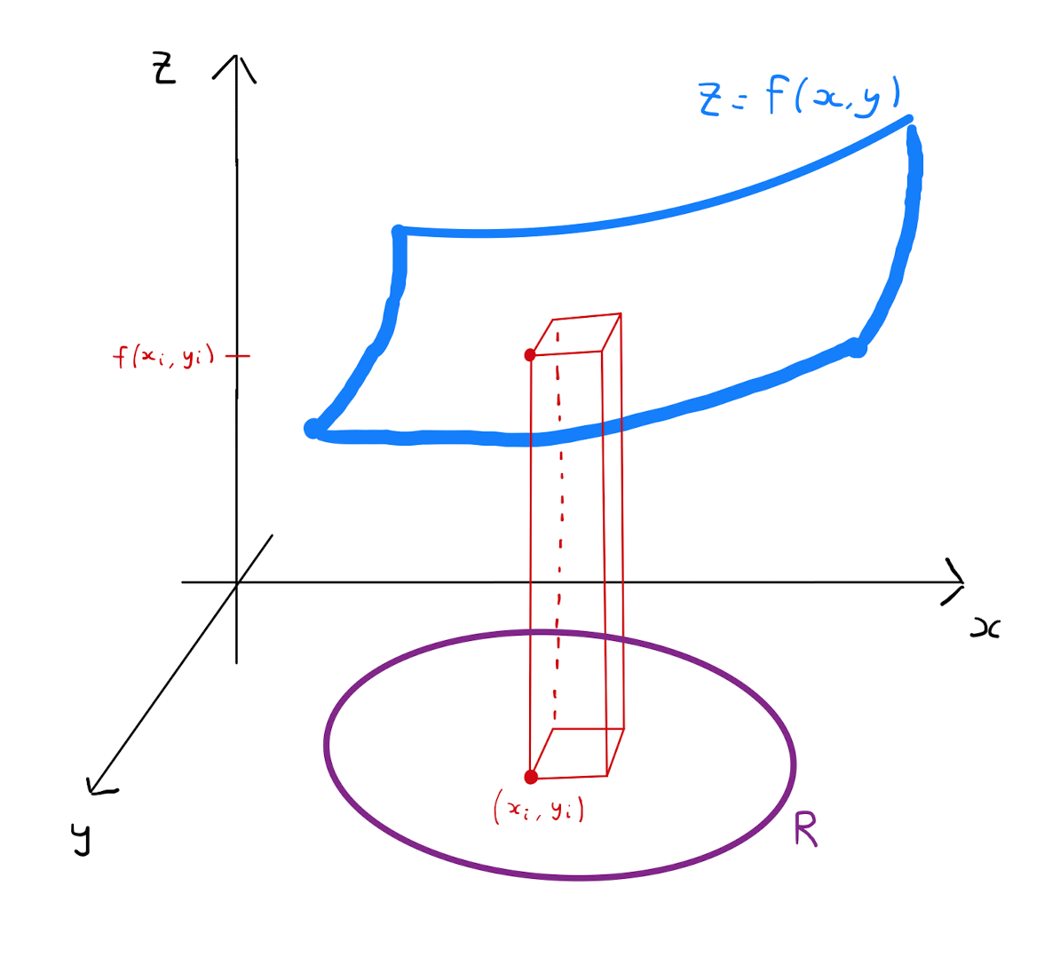
By summing this expression over all rectangular regions \(R_i\), that is \(\sum\limits_{i=0}^{n} f(x_i, y_i) \Delta x \Delta y\), one obtains an approximation of the volume under the surface \(z=f(x,y)\) over the entirety of the region \(R\).
The idea is that in general, though not necessarily, smaller values of \(\Delta x\) and \(\Delta y\) will improve the approximation of the true volume under the surface over \(R\).
Let \(\Delta x\) and \(\Delta y\) tend towards \(0\). If \(\sum\limits_{i=0}^{n} f(x_i, y_i) \Delta x \Delta y\) tends to a finite limit, then this value is the double integral \(\int \int_{R} f(x,y) \,dx \,dy\) of \(f(x,y)\) over the region \(R\). Specifically
\[\int \int_R f(x,y) \,dx \,dy = \lim_{\Delta x, \Delta y \rightarrow 0} \left( \sum\limits_{i=0}^{n} f(x_i, y_i) \Delta x \Delta y \right).\]
11.3 Evaluation of Double Integrals
It is good to have established the formal definition of a double integral seen in Section 11.2. However in practice, computation by this definition would be time-consuming and seems unnecessarily time-consuming. Instead we establish the integration rules and techniques that we are already familiar with. Namely we will show that double integrals can be evaluated as two nested single integrals.
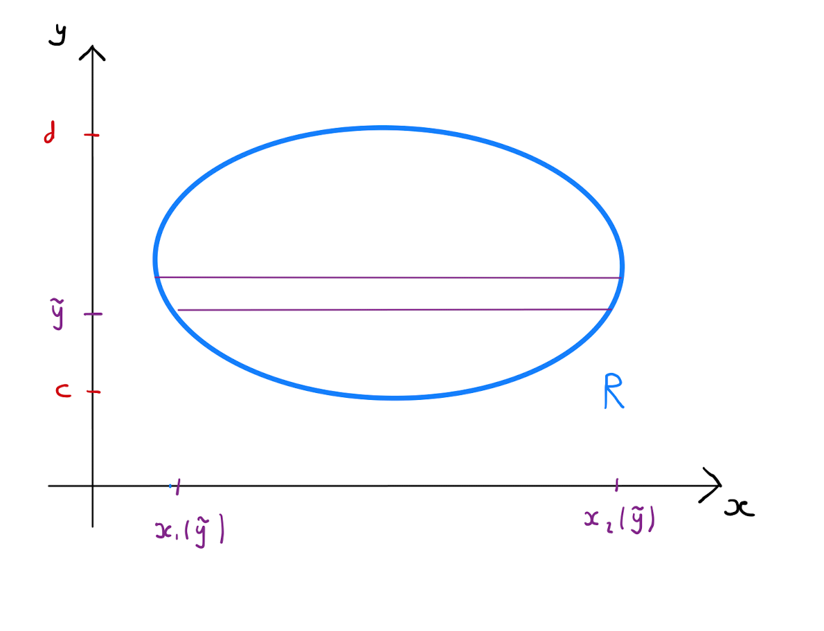
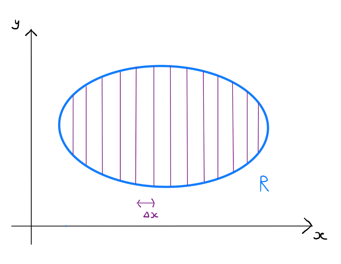
Consider the double integral \(\int \int_R f(x,y) \,dx \,dy\). Let \(c\) be the smallest value that the \(y\)-coordinate takes over the two-dimensional region \(R \subseteq \mathbb{R}^{2}\). Similarly let \(d\) be the largest value that the \(y\)-coordinate takes over \(R\).
Divide the region \(R\) into a collection of \(n\) horizontal strips, each of width \(\Delta y = \frac{d-c}{n}\). The integral of \(f\) over the whole region \(R\) is equal to the sum of the integral over each strip.

Define \(x_1(\tilde{y})\) as the function that returns the smallest value that the \(x\)-coordinate takes over all the points in \(R\) with \(y\)-coordinate equal to \(\tilde{y}\). Similarly define \(x_2(\tilde{y})\) as the function that returns the largest value taken by the \(x\)-coordinate over all the points in \(R\) with \(y\)-coordinate equal to \(\tilde{y}\). It follows that the integral over a typical strip whose baseline has \(y\)-coordinate \(\tilde{y}\) is approximated by \[\int \int_{\text{strip}} f(x,y) \,dx \,dy \approx \Delta y \int_{x_1(\tilde{y})}^{x_2(\tilde{y})} f(x,\tilde{y}) \,dx.\]
Note in the integration on the right hand side that \(\tilde{y}\) is a constant, and the limits of the definite integral replace \(x\) with expressions in terms of \(\tilde{y}\).
Taking the sum over all the strips, one has \[\begin{align*} \int \int_{R} f(x,y) \,dx \,dy &= \sum\limits_{\text{strips}} \left( \int \int_{\text{strip}} f(x,y) \,dx \,dy \right) \\ &\approx \sum\limits_{\text{strips}} \left( \int_{x_1(y)}^{x_2(y)} f(x,y) \,dx \right) \Delta y. \end{align*}\]
Each strip in the summation uniquely determines a value for \(y\) in this approximation, and so \(y\) is treated as a constant in the integration.
Letting \(\Delta y \rightarrow 0\) will cover \(R\) with infinitely many, infinitesimally thin horizontal strips. If \(\sum\limits_{\text{strips}} \left( \int_{x_1(y)}^{x_2(y)} f(x,y) \,dx \right) \Delta y\) tends to a finite limit as \(\Delta y \rightarrow 0\), then \[\sum\limits_{\text{strips}} \left( \int_{x_1(y)}^{x_2(y)} f(x,y) \,dx \right) \Delta y \rightarrow \int_{c}^{d} \int_{x_1(y)}^{x_2(y)} f(x,y) \,dx \,dy,\] and as this happens the approximation of the integral of \(f\) over \(R\) becomes increasingly accurate. Therefore \[\int \int_{R} f(x,y) \,dx \,dy = \int_{c}^{d} \int_{x_1(y)}^{x_2(y)} f(x,y) \,dx \,dy.\]
Writing the double integral as nested single integrals gives us a simple technique by which to calculate double integrals.
Note:
The inner integral, that is the integral with respect to \(x\), should be performed first.
The inner limits \(x_1(y)\) and \(x_2(y)\) depend on \(y\). After performing the first single integral, the function will be univariate in terms of \(y\).
The limits \(c,d\) are constants that ensure the strips cover all of \(R\);
Evaluating double integrals can be difficult, and so the following tips are provided:
Always sketch the region in a large clear diagram.
The main difficulty in these problems is getting the limits of integration correct, particularly \(x_1(y)\) and \(x_2(y)\). Check your chosen expressions evaluate to the correct upper and lower bounds of \(x\) for some fixed \(y\)-coordinate. Your sketch will help you here.
Evaluate \(I = \int \int_R y^2 -2x \,dx \,dy\) where
Start by sketching \(R\):
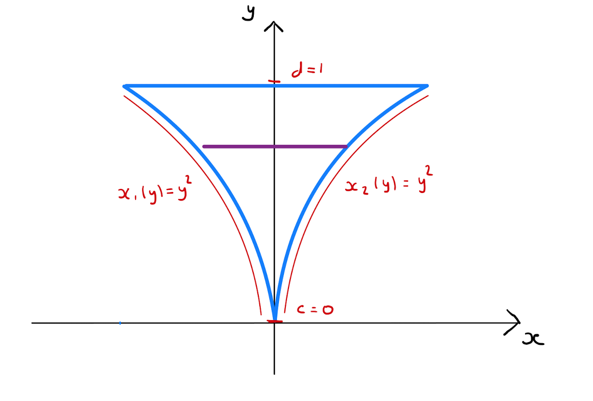
The largest value that the \(y\)-coordinate can take over the region \(R\) is \(1\), therefore set \(d=1\). Similarly the smallest value that the \(y\)-coordinate can take over the region \(R\) is \(0\), so set \(c=0\).
For some fixed value \(y_0\) for the \(y\)-coordinate, the smallest value that the \(x\)-coordinate can take in \(R\) is \(-y_{0}^{2}\). Specifically \(R\) is bounded on the left by the curve \(x=-y^2\). Therefore set \(x_1(y) = - y^2\). Similarly the largest value that the \(x\)-coordinate can take among all points in \(R\) with \(y\)-coordinate \(y_0\) is \(y_0^2\), that is \(R\) is bounded on the right by the curve \(x =y^2\). Therefore set \(x_2(y) = y^2\).
This allows us to formulate the double integral as two nested single integrals, and evaluate:
11.4 Changing Order of Integration
Consider the nested single integrals given by
In attempting to evaluate \(I\), one encounters an immediate problem: there is no explicit function whose derivative with respect to \(x\) is \(e^{x^3}\).
To deal with this type of issue, one can attempt to change the order of integration. Specifically in Example 11.4.1, one wants to perform the integration with respect to \(y\) before the integration with respect to \(x\).
To formulate the double integral \(\int \int_{R} f(x,y) \,dx \,dy\) in this way, one must partition \(R\) into vertical strips rather than horizontal strips.
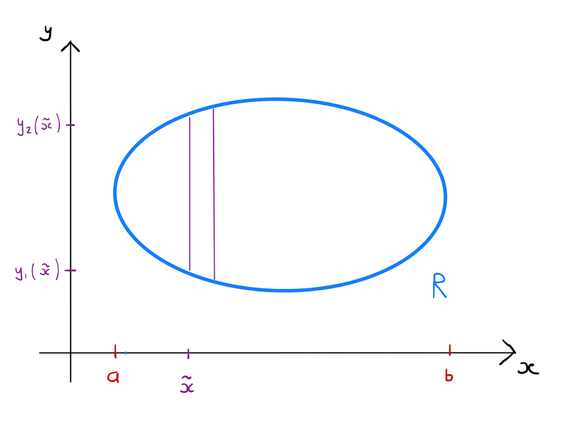
Specifically let \(a\) be the smallest value that the \(x\)-coordinate takes over the two-dimensional region \(R\subseteq \mathbb{R}^{2}\). Similarly let \(b\) be the largest value that the \(x\)-coordinate takes over \(R\). Divide the region \(R\) into a collection of \(n\) vertical strips each width \(\Delta x = \frac{b-a}{n}\). The integral of \(f\) over the whole of \(R\) is equal to the sum of the integral over each strip.
Define \(y_1(\tilde{x})\) as the function that returns the smallest value that \(y\)-coordinate takes over all points in \(R\) with \(x\)-coordinate equal to \(\tilde{x}\). Similarly define \(y_2(\tilde{x})\) as the function that returns the largest value taken by the \(y\)-coordinate over all the points in \(R\) with \(x\)-coordinate equal to \(\tilde{x}\). It follows that the integral over a typical strip bound on the left by the line \(x=\tilde{x}\) is approximated by
Note in the integration on the right hand side that \(\tilde{x}\) is a constant, and the limits of the definite integral replace \(y\) with expressions in terms of \(\tilde{x}\).
Taking the sum over all the strips, one has \[\begin{align*} \int \int_{R} f(x,y) \,dx \,dy &= \sum\limits_{\text{strips}} \left( \int \int_{\text{strip}} f(x,y) \,dx \,dy \right) \\ &\approx \sum\limits_{\text{strips}} \left( \int_{y_1(x)}^{y_2(x)} f(x,y) \,dy \right) \Delta x. \end{align*}\]
Each strip in the summation uniquely determines a value for \(x\) in this approximation, and so \(x\) is treated as a constant in the integration.
Letting \(\Delta x \rightarrow 0\) will cover \(R\) with infinitely many, infinitesimally thin vertical strips. If \(\sum\limits_{\text{strips}} \left( \int_{y_1(x)}^{y_2(x)} f(x,y) \,dy \right) \Delta x\) tends to a finite limit as \(\Delta x \rightarrow 0\), then \[\sum\limits_{\text{strips}} \left( \int_{y_1(x)}^{y_2(x)} f(x,y) \,dy \right) \Delta x \rightarrow \int_{a}^{b} \int_{y_1(x)}^{y_2(x)} f(x,y) \,dy \,dx,\] and as this happens the approximation of the integral of \(f\) over \(R\) becomes increasingly accurate. Therefore \[\int \int_{R} f(x,y) \,dx \,dy = \int_{a}^{b} \int_{y_1(x)}^{y_2(x)} f(x,y) \,dy \,dx.\]
So one has obtained a new technique by which to evaluate double integrals, this time integrating with respect to \(y\) first. Note that
The inner limits \(y_1(x)\) and \(y_2(x)\) depend on \(x\). After performing the first single integral, the function will be univariate in terms of \(x\);
The limits \(a,b\) are constants that ensure the vertical strips cover all of \(R\).
As before when utilising this technique
The region of integration should always be sketched in a large clear diagram;
The main difficulty is getting the limits of integration correct, particularly \(y_1(x)\) and \(y_2(x)\). Check your chosen expressions evaluate to the correct upper and lower bounds of \(y\) for some fixed \(x\)-coordinate. Your sketch will help you here.
With this new technique in mind, one can reattempt to calculate the nested single integrals of Example 11.4.1.
From the expression of \(I\) as single nested integrals where an integration with respect to \(x\) is performed first, we can identify that \(c=0, d=0, x_1(y)=\sqrt{\frac{y}{3}}\) and \(x_2(y)=1\). This allows us to sketch the region of integration:

We seek to reformulate \(I\) as single nested integrals where an integration with respect to \(y\) is performed first. To do this \(R\) is partitioned into vertical strips:

One identifies that \(a=0,b=1, y_1(x)=0\) and \(y_2(x)=3x^2\). Therefore
In general, when formulating nested single integrals for a double integral of a function \(f\) over some two-dimensional region \(R\), it is important to consider which order of integration will be simpler to calculate. This choice might be forced by the function \(f\) as above, but could also be determined by the region \(R\): is it easier to work with \(x_1(y), x_2(y)\) or \(y_1(x), y_2(x)\)?
11.5 Averages and Centroids
The average of a finite number of real values \(a_1, a_2, \ldots, a_n\) is given by
If each value \(a_i\) is given a weight \(w_{i}\), then a weighted average of \(a_i\) for \(i \in \{ 1,\ldots, n \}\), can be defined as
Setting \(w_i=1, \forall i\) recovers the average from the weighted average.
Define
\(a_1\) to be your percentage result in the May/June MATH1006 exam, and \(w_1=0.7\);
\(a_2\) to be your percentage result in the January MATH1006 assessment, and \(w_2=0.08\);
\(a_3\) to be your percentage result in the Spring MATH1006 assessment, and \(w_3=0.07\);
\(a_4\) to be your percentage result in the Core Programming coursework, and \(w_4=0.15\).
Then the weighted average of \(a_1, a_2, a_3, a_4\) is your final MATH1006 result.
Can the notion of an average be extended from a finite discrete list to a more general setting? Specifically one might ask what is the average value \(\bar{f}\) that a function of two real variables \(f(x,y)\) takes over a finite region \(R\) in the \((x,y)\)-plane.
Model the UK as a two-dimensional region \(R\) in the \((x,y)\)-plane. Let \(f(x,y)\) be the amount of rainfall in the location \((x,y)\) in \(R\) over a day. Then the average rainfall in the UK that day can be calculated as the average of \(f(x,y)\) over \(R\).
Let \(f(x,y)\) be a function of two real variables, and \(R\) be a finite region in the \((x,y)\)-plane. Then the average value taken by \(f\) over the region \(R\) is given by
Proof. Let \(\Delta x, \Delta y >0\) be sufficiently small values. Cover the region \(R\) with rectangles \(R_1, R_2, \ldots R_n\) each with a side of length \(\Delta x\) parallel to the \(x\)-axis, and a side of length \(\Delta y\) parallel to the \(y\)-axis.
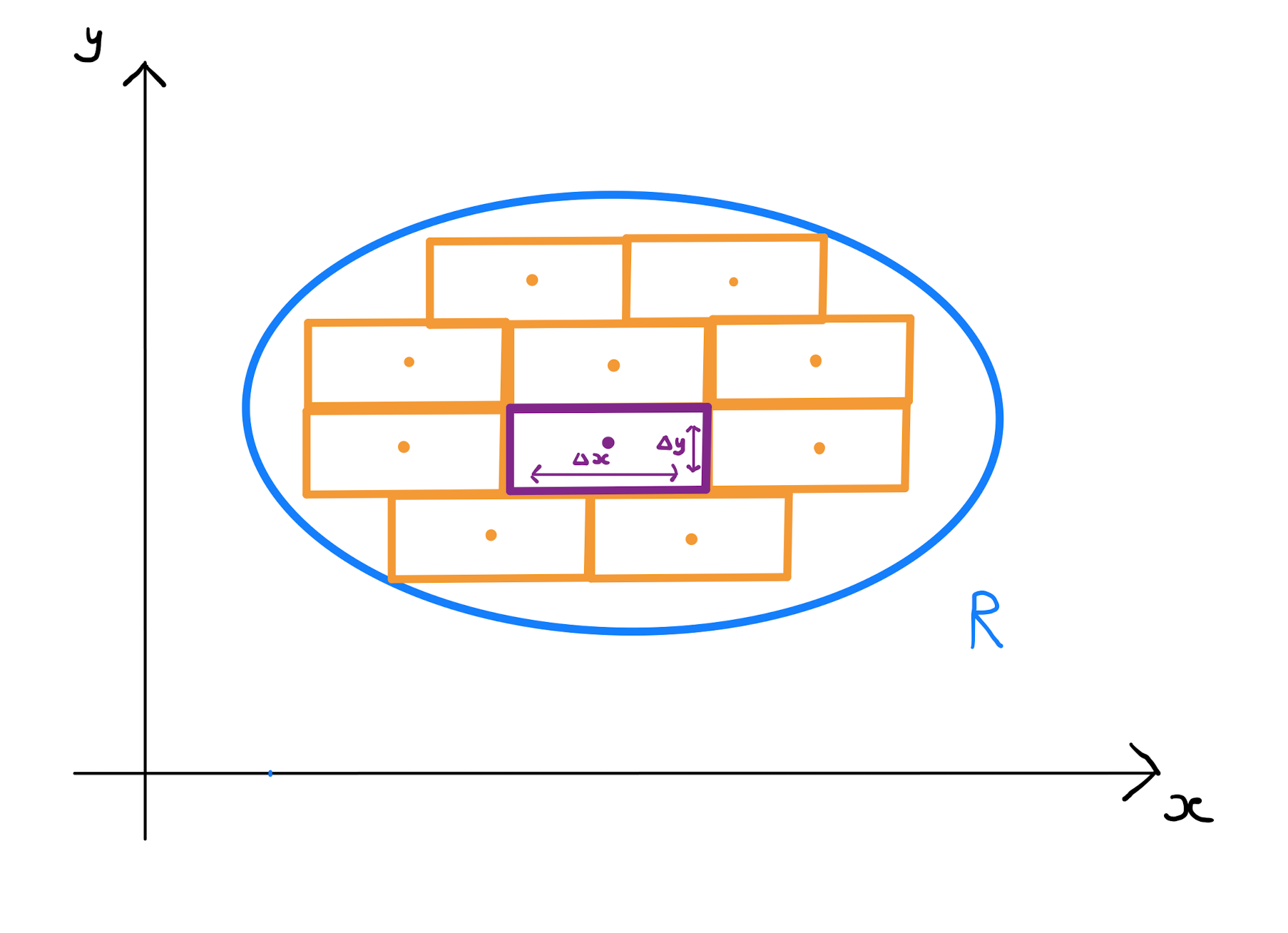
Let \((x_i,y_i)\) be the point at the center of rectangle \(R_{i}\), and define \(f_{i} = f(x_i,y_i), \forall i\). Further let \(w_i = \Delta x \Delta y\). Consider the weighted average of the finite list of the \(f_{i}\):
The numerator of this expression approximates the total value of \(f\) over the entirety of \(R\). The denominator approximates the total area of \(R\). The expression therefore serves as an approximation of the true average \(\bar{f}\) of \(f\) over \(R\).
The limiting process of \(\Delta x, \Delta y \rightarrow 0\) causes the summation over all rectangles to become a double integral over the region \(R\). Furthermore the approximation of \(\bar{f}\) becomes and equality in the limit. The result follows.
The proof of Theorem 11.5.3 is similar to the definition of the double integral.
By setting \(f(x,y)=x\) the average value \(\bar{x}\) that the \(x\)-coordinate takes over the region \(R\) can be calculated. Specifically
Similarly the average \(y\)-coordinate over the region \(R\), denoted \(\bar{y}\), is given by
The centroid or center of mass of a region \(R\) is given by \((\bar{x},\bar{y})\).
Calculate the center of mass of the semi-circle \(R\) given by the set of points \((x,y)\) that satisfy \(x^2 + y^2 \leq 1\) and \(x \geq 0\).
Note that without the need to perform any calculations, one can tell that \(\bar{y}=0\) since the region \(R\) is symmetrical about the \(x\)-axis: each positive value of \(y\) has a corresponding negative value.
To calculate \(\bar{x}\), one needs to calculate \(\int \int_{R} x \,dx \,dy\) and \(\int \int_{R} 1 \,dx \,dy\). The integral \(\int \int_{R} 1 \,dx \,dy\) is the area of \(R\): the area of a semi-circle with radius \(1\) is known to be \(\frac{\pi}{2}\). It remains to calculate \(\int \int_{R} x \,dx \,dy\). Sketch the region \(R\) to calculate necessary bounds for repeated single integrals. We use horizontal strips.
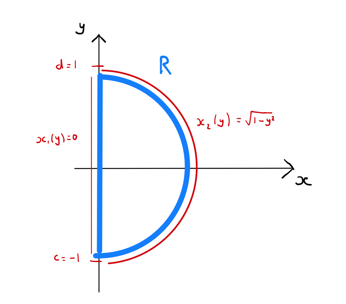
Observe that \(c=-1, d=1, x_1(y)=0\) and \(x_2(y)= \sqrt{1-y^2}\). So calculate that
Therefore
So the centroid is \((\bar{x},\bar{y}) = \left( \frac{4}{3 \pi}, 0 \right)\).