Chapter 2 Coordinates, Curves and Surfaces

A coordinate system on a space is a collection of real variables, each taking values in a specified subset of $\mathbb{R}$, for which every point in the space is described by certain values for the variables.

We are already very familiar with this notion of coordinate systems. For example, one can use two numbers, longitude and latitude, to describe each point uniquely on the surface of the Earth.

Often a problem that is computationally difficult in one coordinate system will miraculously simplify when a move to another coordinate system is made. This is something we will see later in the course.

2.1 Common Two Dimensional Coordinate Systems

In this subsection we study two coordinate systems that can be used to describe the space $\mathbb{R}^{2}$.

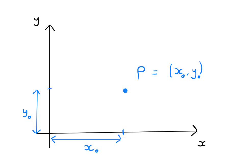
You will already be familiar with Cartesian coordinates: the standard $(x,y)$ coordinates on $\mathbb{R}^{2}$. Specifically two orthogonal coordinate axes lie in $\mathbb{R}^{2}$, the $x$-axis and the $y$-axis. Given a point $P \in \mathbb{R}^2$, the values that $x$ and $y$ take are the distances of $P$ from the two axis including sign. The variables $x$ and $y$ can take any value in $\mathbb{R}$.

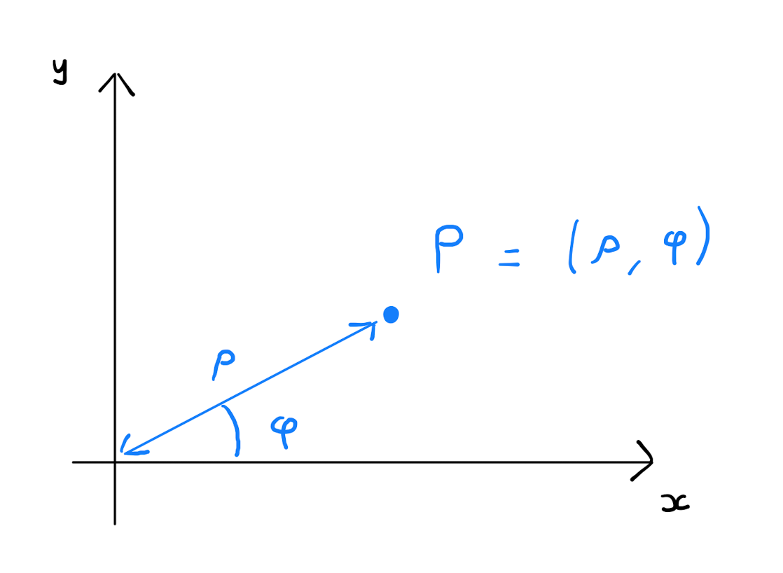
Alternatively one can describe $P$ using polar coordinates. First consider the line segment $OP$ from the origin to $P$. Define $\rho$ to be the length of $OP$, that is, the distance of $P$ from the origin. Note that necessarily $\rho \geq 0$. Define $\varphi$ to be the angle that $OP$ makes with the positive $x$-axis. It follows that $\varphi \in \left[ 0, 2 \pi \right)$. The pair $(\rho, \varphi)$ are the polar coordinates of $P$.

Each point in $\mathbb{R}^{2}$ is uniquely described by values of $\rho$ and $\varphi$, with one exception: the origin. Why?

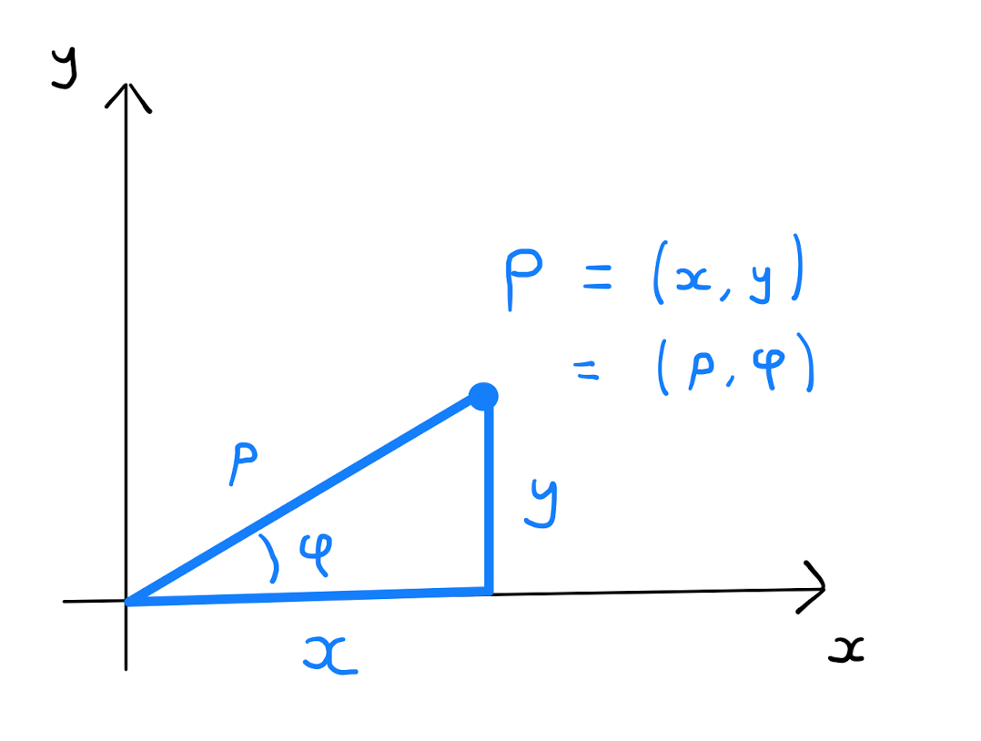
Given a point $P \in \mathbb{R}^2$ described in polar coordinates by $(\rho,\varphi)$, the Cartesian coordinates $(x,y)$ of $P$ are given by \[x = \rho \cos \varphi \qquad \text{and} \qquad y = \rho \sin \varphi.\]

Assume $P$ belongs to the upper right quadrant of $\mathbb{R}^{2}$. The result follow from some simple trigonometric analysis of the following right angle triangle:

The cases of $P$ belong to the other quadrants follow similarly.

Consider the point $P \in \mathbb{R}^{2}$ given in Cartesian coordinates by $(-2,2)$. Convert this point into polar coordinates.

The polar coordinates are given by

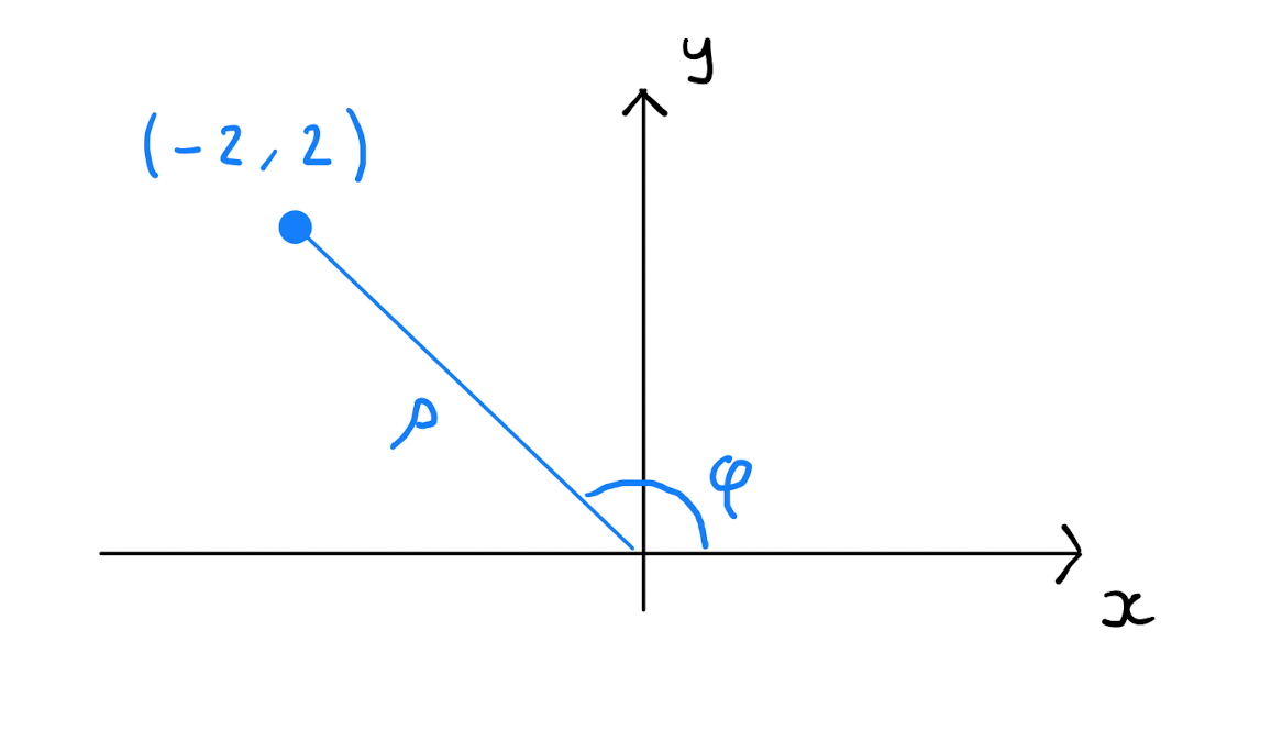
\[\begin{align*} \rho &= \text{Length}(\mathbf{0} P) \\ &= \sqrt{(-2)^2+ 2^2} \\ &= 2, \\[5pt] \varphi &= \text{Angle between }\mathbf{0} P \text{ and the positive $x$-axis} \\ &= \arctan \left( \frac{2}{-2} \right) \\ &= \arctan \left( -1 \right) \\ &= \frac{3\pi}{4}. \end{align*}\]

So $P$ is given by $\left( 2, \frac{3\pi}{4} \right)$ in polar coordinates.

Consider the point $P \in \mathbb{R}^{2}$ given in polar coordinates by $\left( 6,\frac{\pi}{3} \right)$. Convert this point into Cartesian coordinates.

By Theorem 2.1.1, the Cartesian coordinates are given by

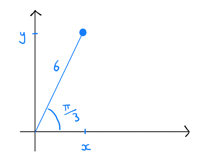
\[\begin{align*} x &= 6 \cos \left( \frac{\pi}{3} \right) = 6 \cdot \frac{1}{2} = 3, \\ y &= 6 \sin \left( \frac{\pi}{3} \right) = 6 \cdot \frac{\sqrt{3}}{2} = 3\sqrt{3}. \end{align*}\]

So $P$ is given by $\left( 3, 3\sqrt{3} \right)$ in Cartesian coordinates.

2.2 Common Three Dimensional Coordinate Systems

There are three coordinate systems that are commonly used in $\mathbb{R}^{3}$.

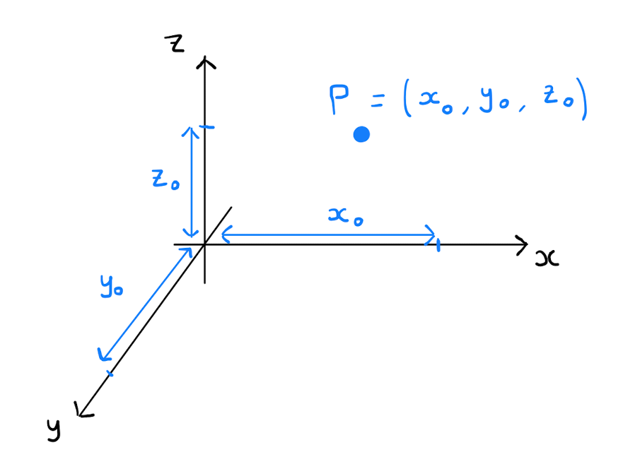
The first of these is again the commonly used Cartesian coorinates: the standard $(x,y,z)$ coordinates in $\mathbb{R}^{3}$. Specifically there are three pairwise ortogonal axes in $\mathbb{R}^{3}$: the $x$-axis, the $y$-axis and the $z$-axis. Given a point $P \in \mathbb{R}^{3}$, the $x$ coordinate is defined as the distance of $P$ from the $(x,y)$-plane, the $y$ coordinate is defined as the distance of $P$ from the $(x,z)$-plane and the $z$ coordinate is defined as the distance of $P$ from the $(y,z)$-plane. Each point $P \in \mathbb{R}^{3}$ is determined uniquely by its’ Cartesian coordinates.

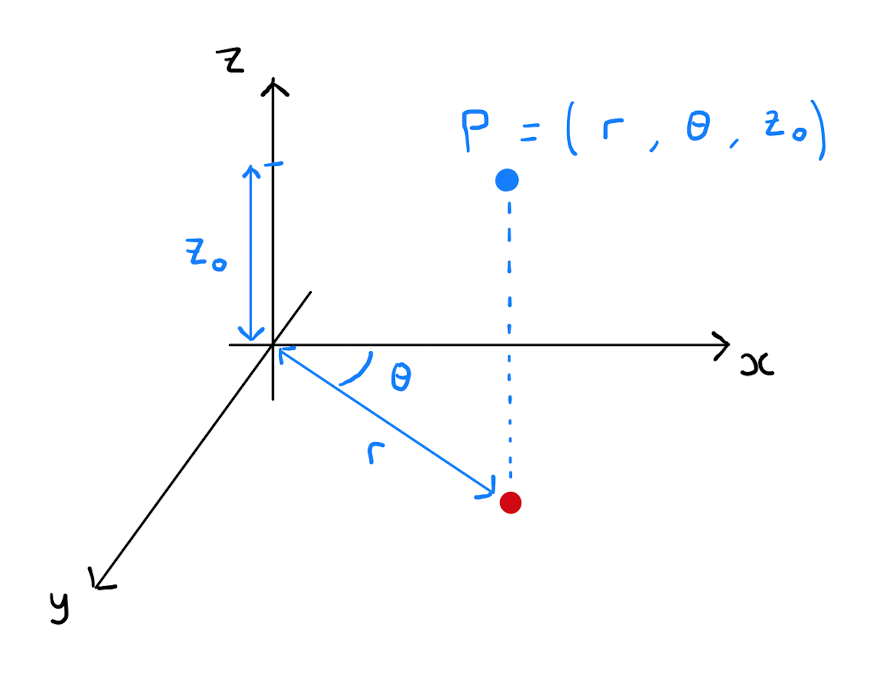
Alternatively one can describe $P$ using cylindrical coordinates, which consists of a triple $(\rho, \varphi, z)$. Cylindrical coordinates are to some extent an extension of polar coordinates. The coordinates $(\rho,\varphi)$ are the polar coordinates that describe the point $(x,y)$ in the $(x,y)$-plane. The $z$-coordinate remains as in Cartesian coordinates.

Cylindrical coordinates are so called as cylinders are easily described in cylindrical coordinates by a constant value for the coordinate $\rho$. If you are working on a problem that appears cylindrical in some sense, then switching to cylindrical coordinates may simplify the problem greatly.

Given a point $P \in \mathbb{R}^{3}$ described in cylindrical coordinates by $(\rho,\varphi, z)$, the Cartesian coordinates $(x,y,z)$ of $P$ are given by \[\left( x,y,z \right) = \left( \rho \cos \varphi, \rho \sin \varphi, z \right).\]

Finally one can describe $P$ using spherical coordinates. First consider the line segment $OP$ from the origin to $P$. Define $r$ to be the length of $OP$, that is, the distance of $P$ from the origin. Note that necessarily $r \geq 0$. Define $\theta$ to be the angle that $OP$ makes with the positive $z$-axis. It follows that $\theta \in \left[ 0 , \pi \right]$. Define $\phi$ to be the angle that $OP$ makes with the positive $x$-axis in the $(x,y)$-plane. It follows that $\phi \in \left[ 0 , 2\pi \right)$. The triple $(r, \theta, \phi)$ are the spherical coordinates of $P$.

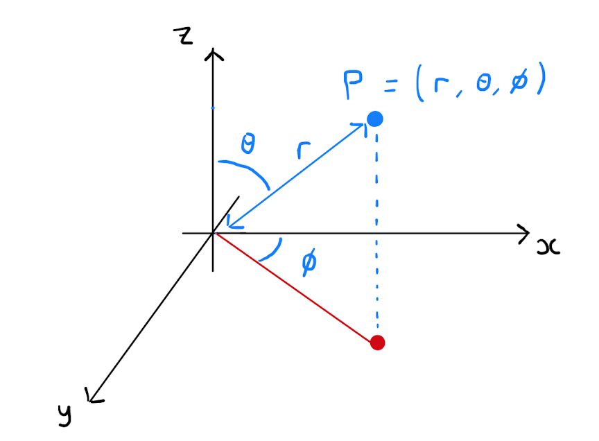
Spherical coordinates are so called as spheres are easily described in spherical coordinates by a constant value for the coordinate $r$. Similarly to previously, if you are working on a problem that appears spherical in some sense, then switching to spherical coordinates can simplify the problem greatly.

Given a point $P \in \mathbb{R}^{3}$ described in spherical coordinates by $(r,\theta, \phi)$, the Cartesian coordinates $(x,y,z)$ of $P$ are given by \[\left( x,y,z \right) = \left( r \sin \theta \cos \phi, r \sin \theta \sin \phi, r \cos \theta \right).\]

Consider the point $P \in \mathbb{R}^{3}$ given in spherical coordinates by $\left( 4, \frac{3 \pi}{4}, \frac{\pi}{3} \right)$. Convert this point into Cartesian coordinates.

By Theorem 2.2.2, the Cartesian coordinates are given by

\[\begin{align*} x &= 4 \sin \left( \frac{3 \pi}{4} \right) \cos \left( \frac{\pi}{3} \right) = \sqrt{2}, \\ y &= 4 \sin \left( \frac{3 \pi}{4} \right) \sin \left( \frac{\pi}{3} \right) = \sqrt{6}, \\ z &= 4 \cos \left( \frac{3 \pi}{4} \right) = -2 \sqrt{2}. \end{align*}\]

So $P$ is given by $\left( \sqrt{2}, \sqrt{6}, -2 \sqrt{2} \right)$ in Cartesian coordinates.

2.3 Curves in Parametric Form

Until now, we have described curves and surfaces in $\mathbb{R}^{2}$ or $\mathbb{R}^{3}$ as the set of points satisfying some condition: usually an equation. It is often preferable to describe these objects instead in parametric coordinates.

Let $x=x(t)$ and $y=y(t)$ be two continuous functions of $t$ for $t \in I$, where $I \subset \mathbb{R}$. The set of points \[\Big\{ P = \big( x(t), y(t) \big) \in \mathbb{R}^{2} : t \in I \Big\}\] is a parametric curve. The functions $x(t)$ and $y(t)$ are called parametric equations, and $t$ is called the parameter.

To describe a curve using parametric coordinates, not only do we use variables representing the Cartesian coordinates $x$ and $y$ in $\mathbb{R}^{2}$, we introduce a third variable $t$ which can take values in some fixed subset $I$ of $\mathbb{R}$. The coordinates $x$ and $y$ are then described as a function of $t$: $x(t)$ and $y(t)$ respectively. As the value of $t$ moves through $I$, the point $P=(x(t), y(t))$ draws a curve in $\mathbb{R}^{2}$.

Defintion 2.3.1 generalises easily to a curve in $\mathbb{R}^{3}$ by introducing a third coordinate $z=z(t)$.

Usually parametric curves are described in vector form using a position vector $\mathbf{r}$ which depends on $t$, written $\mathbf{r}(t)$. More specifically $\mathbf{r}(t) = \big( x(t), y(t) \big)$ or $\mathbf{r}(t) = \big( x(t), y(t), z(t) \big)$.

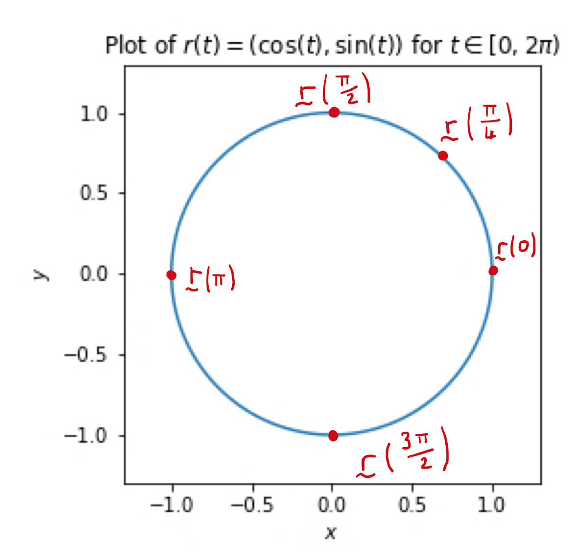
Consider the parametric curve in $\mathbb{R}^{2}$ described by $\mathbf{r}(t) = (\cos (t), \sin (t))$, for $t \in \left[ 0,2 \pi \right)$. This parametric curve describes a circle.

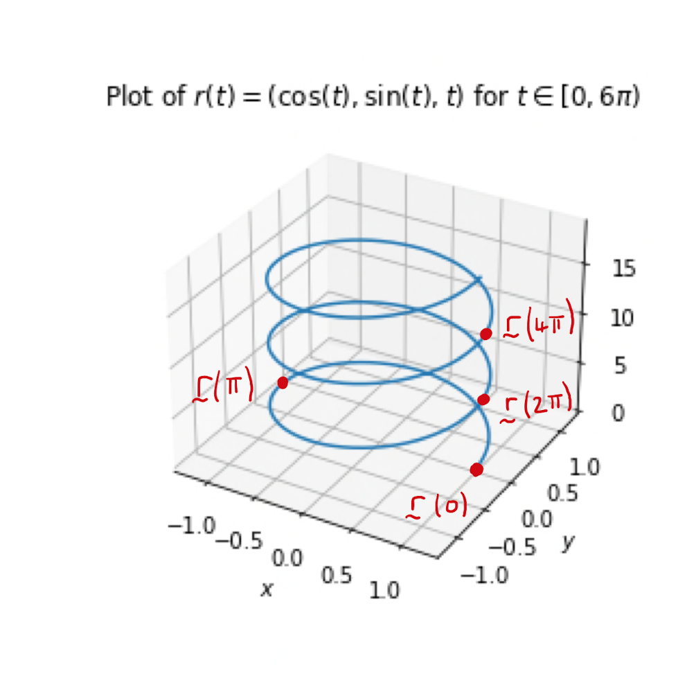
Consider the parametric curve in $\mathbb{R}^{3}$ described by $\mathbf{r}(t) = (\cos (t), \sin (t),t)$, for $t \in \mathbb{R}_{>0}$. Note that restricting to the $(x,y)$-plane, replicates the parametric circle of Example 2.3.2. However the $z$-coordinate increases at a constant rate with $t$. Hence the parametric curve describes a circular spiral.

One might ask how to find the tangent vector to a parametric curve. For a curve of the form $y=f(x)$, the tangent line is found via differentiation. Specifically the gradient of the tangent line is given by $\frac{d y}{d x} = f'(x)$. Differentiation also features heavily in answering this question in the parametric setting.

A parameterisation $\mathbf{r}(t) = (x(t), y(t))$ or $\mathbf{r}(t) = (x(t), y(t),z(t))$ is differentiable if each component is differentiable as a function of $t$, that is, $x(t),y(t)$ and $z(t)$ are differentiable. Furthermore the derivative of a vector function of one variable is found by differentiating component-wise. For example \[\begin{align*} &\mathbf{r}(t) = (x(t), y(t)) \\[3pt] \implies \qquad &\frac{d \mathbf{r}(t)}{d t} = \left( \frac{d x}{d t}(t), \frac{d y}{d t}(t) \right). \end{align*}\] and \[\begin{align*} &\mathbf{r}(t) = (x(t), y(t), z(t)) \\[3pt] \implies \qquad &\frac{d \mathbf{r}(t)}{\partial t} = \left( \frac{dx}{dt}(t), \frac{dy}{dt}(t), \frac{dz}{dt}(t) \right). \end{align*}\] where $\frac{dx}{dt} = \lim_{\Delta t \rightarrow 0} \frac{x(t + \Delta t) - x(t)}{\Delta t}$, etc.

Let $C$ be the curve given by the continuously differentiable parametrisation $\mathbf{r}(t)$ for a set of values of $t$. Then $\frac{d\mathbf{r}(t)}{dt}$ is a tangent vector to the curve at $\mathbf{r}(t)$.

Assume that $C$ is contained in $\mathbb{R}^{2}$. The case where $C \subset \mathbb{R}^{3}$ will follow an almost identical argument. For some fixed value of $t$, let $P$ be the point on $C$ at $\mathbf{r}(t)$, and let $Q$ be the point on $C$ at $\mathbf{r}(t + \Delta t)$, where $\Delta t$ is some small non-zero value.

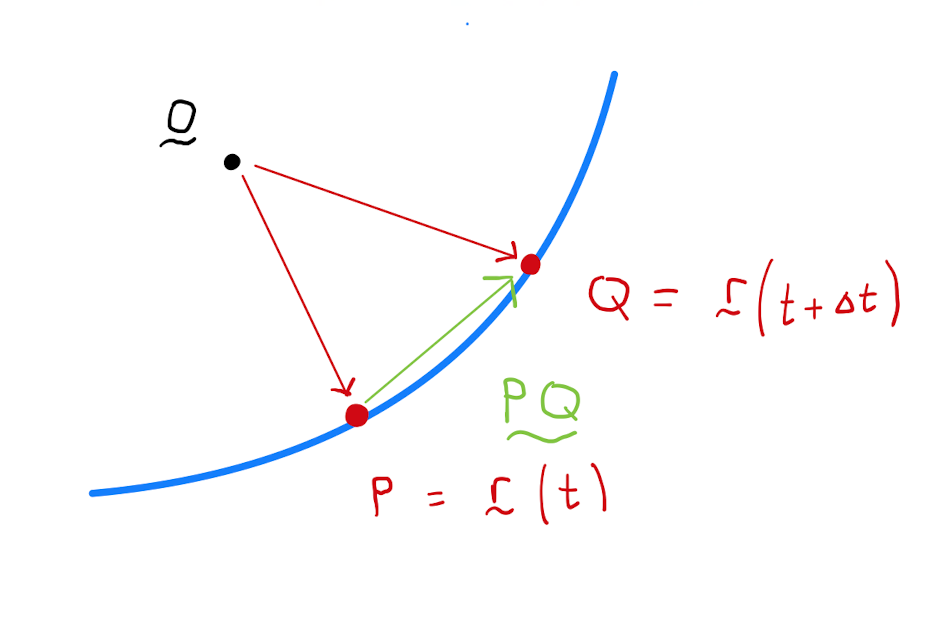
Calculate that

\[\begin{align*} \frac{d \mathbf{r}(t)}{dt} &= \left( \frac{dx}{dt}(t), \frac{dy}{dt}(t) \right) \\ &= \left( \lim_{\Delta t \rightarrow 0} \frac{x(t + \Delta t) - x(t)}{\Delta t}, \lim_{\Delta t \rightarrow 0} \frac{y(t + \Delta t) - y(t)}{\Delta t} \right) \\ &= \lim_{\Delta t \rightarrow 0} \frac{\mathbf{r}(t + \Delta t) - \mathbf{r}(t)}{\Delta t} \\ &= \lim_{\Delta t \rightarrow 0} \frac{PQ}{\Delta t} \end{align*}\]

Note that $\frac{PQ}{\Delta t}$ is a scalar multiple of the vector $PQ$. As $\Delta t \rightarrow 0$, the direction of $PQ$ approaches the direction of the tangent vector at $P$ to $C$.

2.4 Surfaces in Parametric Form

Surfaces in $\mathbb{R}^{3}$ can also be describing in parametric form:

Let $x=x(u,v), y=y(u,v)$ and $z=z(u,v)$ be continuous functions in two variables $u$ and $v$, for $u$ and $v$ in some fixed domain $D \subseteq \mathbb{R}^{2}$. The set of points \[\Big\{ P = \big( x(u,v), y(u,v), z(u,v) \big) \in \mathbb{R}^{3} : (u,v) \in D \Big\}\] is a parametric surface. The functions $x(u,v), y(u,v)$ and $z(u,v)$ are called parametric equations, and $u$ and $v$ are called the parameters.

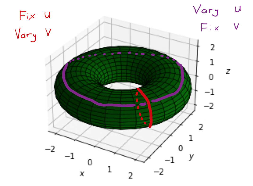
As $u$ varies but $v$ stays constant, the point $P =\left( x(u,v), y(u,v), z(u,v) \right)$ will vary tracing out a curve in $\mathbb{R}^{3}$, exactly as per Defintion 2.3.1. This is similarly true as $v$ varies but $u$ stays constant.

From here, it is easy to see that as $u$ and $v$ are both allowed to vary, that $P$ will trace out a surface.

Similarly to curves, parametric surfaces are often written in vector format: \[\mathbf{r}(u,v) = \big( x(u,v), y(u,v), z(u,v) \big).\]

Consider the parametric surface in $\mathbb{R}^{3}$ described by \[\mathbf{r}(t) = \big( \cos (u) \sin v, \sin (u) \sin(v), \cos(v) \big),\] for $u \in \left[ 0,2 \pi \right)$ and $v \in [0,\pi]$. This parametric surface describes a sphere of radius $1$ centered on the origin. Indeed one can verify that $x^2 + y^2 + z^2 = 1$ for all values of $u$ and $v$.

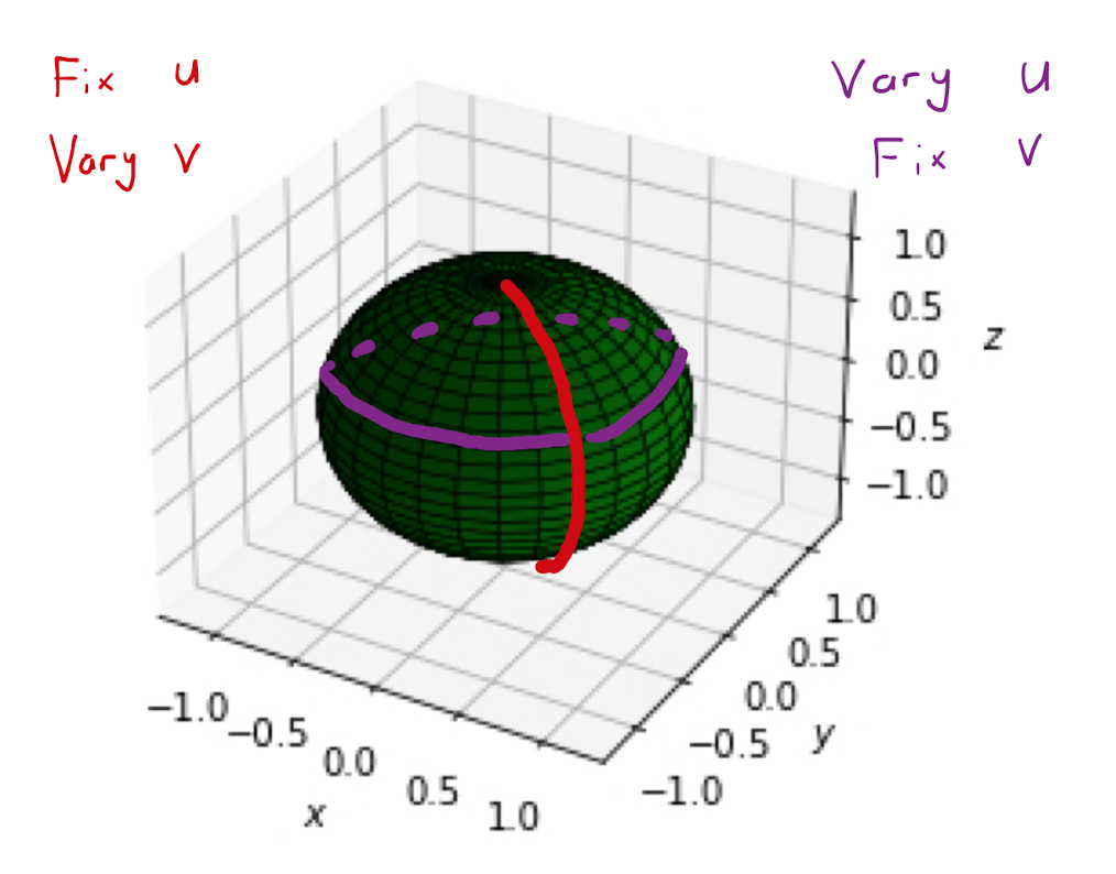
Fixing the value of $v$ as $v_0$ and continuing to vary $u$, restricts the parameterisation $r(u,v_0)$ to one parameter, and subsequently describes a curve on the surface: a circle of latitude. Similarly fixing $u$ as $u_0$, and allowing $v$ to vary, describes a semi-circle of longitude on the sphere.

Let $a,b$ be constants such that $b>a$. Consider the parametric surface in $\mathbb{R}^{3}$ described by \[\mathbf{r}(t) = \Big( \big( b+a \cos(u) \big) \cos(v) , \big( b+a \cos(u) \big) \sin(v), a\sin(u) \Big),\] for $u \in \left[ 0,2 \pi \right]$ and $v \in [0,2 \pi]$. This parametric surface describes a torus, that is, the surface of a donut.