Chapter 3 Limits and Continuity
3.1 Recap: limits for one variable Function
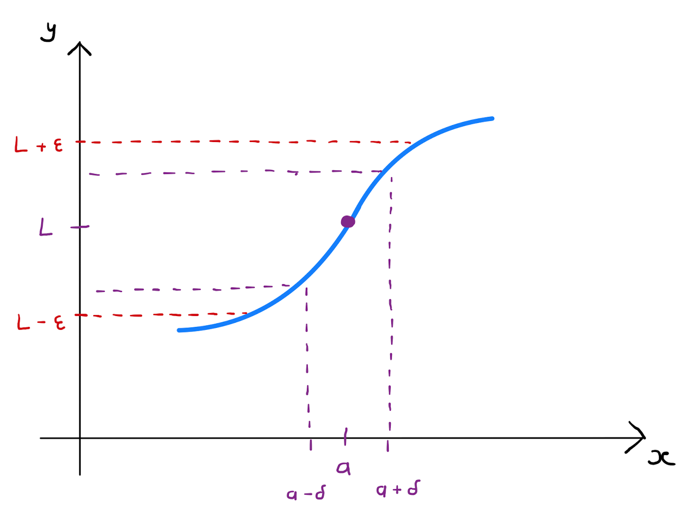
In the Autumn term, we saw the definition of a limit for a univariate function of one variable. The function \(f(x)\) tending to \(L\), denoted \(\lim_{x \rightarrow a} f(x) = L\), means that the limit of \(f(x)\) as \(x\) tends to \(a\) from below and the limit of \(f(x)\) as \(x\) tends to \(a\) from above are both equal to \(L\).
The formal definition, known as the \(\epsilon-\delta\) definition, is that given any \(\epsilon >0\), there exists \(\delta >0\) such that \(\lvert f(x) - L \rvert < \epsilon\), for all \(x\) with \(\lvert x-a \rvert < \delta\).
Furthermore, the function \(f(x)\) is continuous at \(x=a\) of the limit exists at this point, and equals \(f(a)\).
In this section we will generalise this theory to a function of two variables.
3.2 Graphical Introduction to Limits
Consider a function
\[f: D \rightarrow \mathbb{R}\]
where \(D\) is some region in \(\mathbb{R}^{2}\). This function can be represented graphically by a surface as in Chapter 1. Let \((a,b) \in \mathbb{R}^{2}\) such that some circular region centered on \((a,b)\) is contained entirely within \(D\), with the possible exception of the point \((a,b)\).
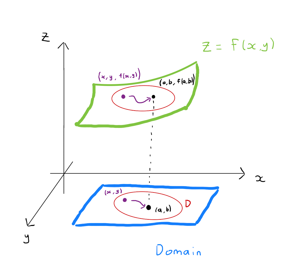
Consider \((x,y) \in D\) that approaches \((a,b)\) becoming infinitely close, but never equal to \((a,b)\). This could happen in a continuous fashion along a suitable curve, or via a sequence of discrete points. One may ask about the behaviour of the point \(P = \big( x,y, f(x,y) \big)\) on the surface as the coordinates \((x,y)\) approach \((a,b)\). There are three distinct possibilities:
1.) For all possible ways that \((x,y)\) approaches \((a,b)\) then the value \(f(x,y)\) tends to the same value \(l\), that is, \(P = \big( x,y, f(x,y) \big)\) approaches \((a,b,l)\). Furthermore the point \((a,b) \in D\), and \(f(a,b)=l\). In this case, one says that \(f\) is continuous and that the limit exists as \((x,y)\) tends to \((a,b)\). This is denoted by \(\lim_{(x,y)\rightarrow (a,b)} f(x,y) = l\).
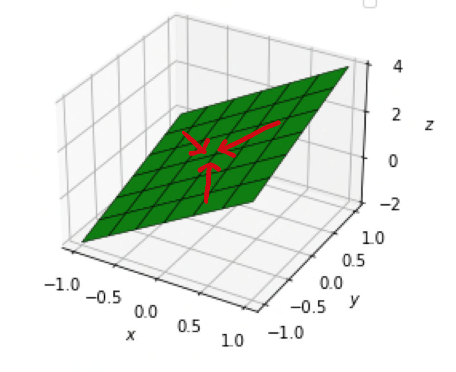
Let \((x,y) \in \mathbb{R}^{2}\) be a point that is not equal to \((0,0)\), but does tend towards the \((0,0)\). Then \[\begin{align*} \lim_{(x,y) \rightarrow (0,0)} f(x,y) &= \lim_{(x,y) \rightarrow (0,0)} 1 + 2x + y \\ &= \lim_{(x,y) \rightarrow (0,0)} (1) + \lim_{(x,y) \rightarrow (0,0)} (2x) + \lim_{(x,y) \rightarrow (0,0)} (y) \\ &= 1 + 0 + 0 \\ &= f(0,0) \\ &= 1. \end{align*}\] This is therefore an example of a function that belongs to Case 1.).
2.) For all possible ways that \((x,y)\) approaches \((a,b)\) then the value \(f(x,y)\) tends to the same value \(l\), that is, \(P = \big( x,y, f(x,y) \big)\) approaches \((a,b,l)\). However \((a,b)\) does not necessarily belong to \(D\), and if indeed \((a,b)\) does belong to \(D\), then \(f(a,b) \neq l\). One still says that the limit exists, denoted \(f(x,y) \rightarrow l\) as \((x,y) \rightarrow (a,b)\), however \(f\) is now said to be discontinuous at \((a,b)\).
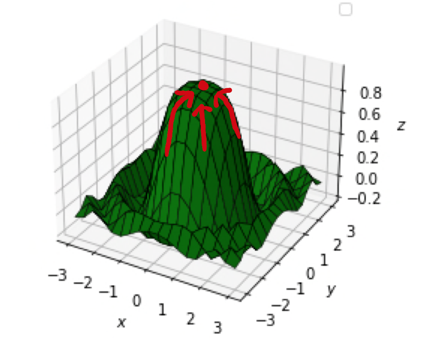
Let \((x,y) \in \mathbb{R}^{2}\) be a point that is not equal to \((0,0)\), but does tend towards the \((0,0)\). Then \[\begin{align*} \lim_{(x,y) \rightarrow (0,0)} f(x,y) &= \lim_{(x,y) \rightarrow (0,0)} \frac{\sin (x^2 + y^2)}{x^2 + y^2} \\ &= \lim_{t \rightarrow 0} \frac{\sin (t)}{t}, \qquad \qquad \qquad \qquad \text{where } t = x^2 + y^2, \\ &= 1, \qquad \qquad \qquad \qquad \qquad \qquad \text{for sufficiently small } t \text{ as } (x,y) \rightarrow 0, \\ &\neq f(0,0) \\ &= 0. \end{align*}\] This is therefore an example of a function that belongs to Case 2.).
3.) The value that \(f(x,y)\) tends to varies dependent on the approach of \((x,y)\) towards \((a,b)\). One says that there does not exist a limit.
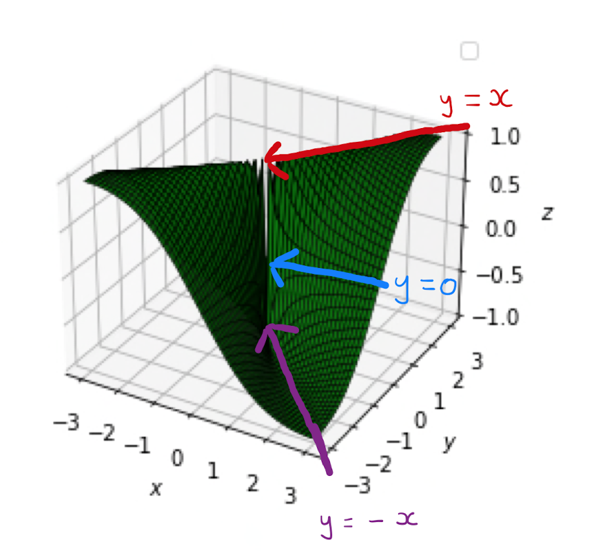
Consider points of the form \((t,0)\) as \(t\) tends towards zero: \[ \lim_{t \rightarrow 0} f(t,0) = \lim_{t \rightarrow 0} \frac{0}{t^2} = 0. \] Alternatively consider points of the form \((t,t)\) as \(t\) tends towards zero: \[ \lim_{t \rightarrow 0} f(t,t) = \lim_{t \rightarrow 0} \frac{2t^2}{2t^2} = 1.\] Since these two limits do not agree, this is an example of a function that belongs to Case 3.).
We will see formal definitions of the two concepts of limits and continuity in the upcoming sections.
3.3 Formal Definition of Limits
Section 3.2 provided an informal approach to limits, considering the problem from a mostly graphical perspective. The word approach was frequently used, and indeed was central to the discussion of cases, however a precise formal mathematical definition of approach is not given. This means we do not yet have a formal mathematical definition of a limit. The following definition of a limit, known as the \(\epsilon-\delta\) definition of a limit is unambiguous and testable for a function of two variables.
One says \(f(x,y)\) has limit \(l\) as \((x,y)\) approaches \((a,b)\) if given any \(\epsilon >0\), we can find \(\delta>0\) such that \[ \lvert f(x,y) - l \rvert < \epsilon, \qquad \text{if } 0 < \lvert (x,y) - (a,b) \rvert < \delta.\]
Here \(\lvert (x,y) - (a,b) \rvert\) is the distance between the two points \((x,y)\) and \((a,b)\), specifically: \[ (x,y) - (a,b) = \sqrt{(x-a)^2 + (y-b)^2}.\] Since it is specified that \(0 < \lvert (x,y) - (a,b) \rvert\), the value of \(f(x,y)\) at \((a,b)\) itself does not play a role in the definition.
There are similarities between the univariate definition of a limit, and the definition for a function of two variables.
An informal interpretation of what it means to show a limit of a function exists at \((a,b)\) is as follows: I will choose some positive value of \(\epsilon\) for which I expect \(f(x,y)\) to be that close to \(l\). You do not know what value of \(\epsilon\) that I will choose, but irrespectively your job is to retort with some specific value for \(\delta\), possibly in terms of the unknown \(\epsilon\), such that provided \((x,y)\) and \((a,b)\) are within \(\delta\) of each other and are distinct, then my wish of \(f(x,y)\) and \(l\) being within \(\epsilon\) of each other is fulfilled.
Consider the function \(f(x,y) = x^2 + 2y^2\). Show that \(f(x,y)\) tends to the limit \(0\) as \((x,y) \rightarrow (0,0)\).
Let \(\epsilon >0\). Choose \(\delta = \sqrt{\frac{\epsilon}{2}}\). Suppose \(0 < \lvert (x,y) - (0,0) \rvert = \lvert (x,y) \rvert < \delta\). Then \[\begin{align*} \lvert f(x,y) - 0 \rvert &= \lvert f(x,y) \rvert \\ &= \lvert x^2 + 2 y^2 \rvert \\ =& x^2 + 2y^2 \\ &\leq 2 \left( x^2 + y^2 \right) \\ &= 2 \lvert (x,y) \rvert \\ &< 2 \delta^2 \\ &= 2 \left( \sqrt{\frac{\epsilon}{2}} \right) ^{2} \\ &= \epsilon \end{align*}\]
Note how closely the example answer follows the logic of Definition 3.3.1. It may appear that \(\delta\) was chosen without explanation. Some rough work will have been completed on the side prior to writing up to find the expression for \(\delta\) that ensures that the sequence of inequalities terminates with \(< \epsilon\) as required.
3.4 Continuity
The formal definition of continuity follows from the definition of a limit, as it did in Section 3.2.
The function \(f\) is continuous at \((a,b)\) if \((a,b)\) belongs to the domain of \(f\), and \[ \lim_{(x,y) \rightarrow (a,b)} f(x,y) = f(a,b).\]
Consider the function
We can calculate that
\(\lim_{(x,y) \rightarrow (0,0)} g(x,y) = 1\);
\(g(0,0) = 1\).
Hence \(g\) is continuous at \((0,0)\).
It is important to compare Example 3.2.2 and Example 3.4.1.