Chapter 12 Jacobian

12.1 Change of variables in the integral of a univariate function

Consider the definite integral of some univariate function \(f(x)\) given by \[I = \int_{x_1}^{x_2} f(x) \,dx.\] Suppose further that \(x\) is a function of \(t\), that is \(x=g(t)\), where \(g\) is injective, \(g'\) is continuous and \(g^{-1}\) is differentiable. In the Autumn semester we saw how to rewrite \(I\) in terms of \(t\) rather than \(x\). In particular, there are three steps to rewriting this general integral:

Rewrite the function to be integrated in terms of \(t\) by replacing every occurrence of \(x\) with \(g(t)\);
Rearranging \(\frac{dx}{dt} = g'(t)\), obtain \(\,dx = g'(t) \,dt\). Use this identity to write \(\,dx\) in terms of \(\,dt\) in \(I\);
Replace the limits \(x_1,x_2\) of \(I\) by \(t_1, t_2\) respectively where \(t_{1} = g^{-1}(x_1)\) and \(t_{2} = g^{-1}(x_2)\).

As a result \[I=\int_{g^{-1}(x_1)}^{g^{-1}(x_2)} f(g(t)) \cdot g'(t) \,dt.\]

The aim of this chapter is to generalise this theory to a real function of two variables.

12.2 Jacobian

Consider \(x,y\) given in terms of \(u,v\) by \[\begin{align*} x &= x(u,v), \\ y &= y(u,v). \end{align*}\] Further suppose this transformation is one-to-one, that is any one pair \((x_0,y_0)\) is obtained uniquely from some pair \((u_0,v_0)\), and similarly each pair \((u_0,v_0)\) determines exactly one pair \((x_0,y_0)\). This transform has an inverse: \[\begin{align*} u &= u(x,y), \\ v &= v(x,y). \end{align*}\]

Let \(f(x,y)\) be a function of \(x\) and \(y\), and let \(R\) be some region in the \((x,y)\)-plane. Consider the integral \[I = \int \int_{R} f(x,y) \,dx \,dy.\] How is \(I\) given in terms of \(u\) and \(v\)? The three steps followed for a univariate change of variables of an integral must be followed again in this multivariate setting.

The function \(f(x,y)\) being integrated must be written in terms of \(u\) and \(v\);
The region \(R\) must be understood in terms of \(u,v\);
The differentials \(\,dx \,dy\) must be rewritten in terms of \(\,du \,dv\).

The first two steps are relatively straightforward. The function \(f(x,y)\) can be written in terms of \(u\) and \(v\), by replacing every occurance of \(x\) or \(y\) by \(x(u,v)\) or \(y(u,v)\) respectively. The region \(R\) is replaced by the region \(S\) belonging to the \((u,v)\)-plane defined as the inverse image of \(R\) under the transformation. Formally \[S = \left\{ (u_0,v_0) : (x_0,y_0) = \big(x(u_0,v_0), y(u_0,v_0) \big) \in R \right\}.\]

On the other hand, the third step is more involved and requires us to study the Jacobian of the transformation.

When defining the double integral \(I= \int \int_{R} f(x,y) \,dx \,dy\), the region \(R\) was partitioned into small rectangles of length \(\Delta x\) and width \(\Delta y\). The integral \(I\) was then approximated by \[I \approx \sum\limits_{\text{rectangles}} f(x,y) \Delta x \Delta y.\] However there is no intrinsic reason to use rectangles. Indeed any subdivision of \(R\) into small consistently-shaped sub-regions will do.

Consider a subdivision of \(R\) into small areas defined by families of the level curves of \(u(x,y)\) and \(v(x,y)\). Specifically fix two small positive values \(\Delta u\) and \(\Delta v\). Further fix values \(u_0,v_0\), and consider the area \(A\) bounded by the lines \(u(x,y)=u_0\), \(u(x,y)=u_0 + \Delta u\), \(v(x,y)=v_0\) and \(v(x,y)=v_0 + \Delta v\). Denote the area of \(A\) by \(\Delta A\).

The quantity \(\Delta A\) is called the area element.

The region \(R\) can be partitioned with copies of \(A\).

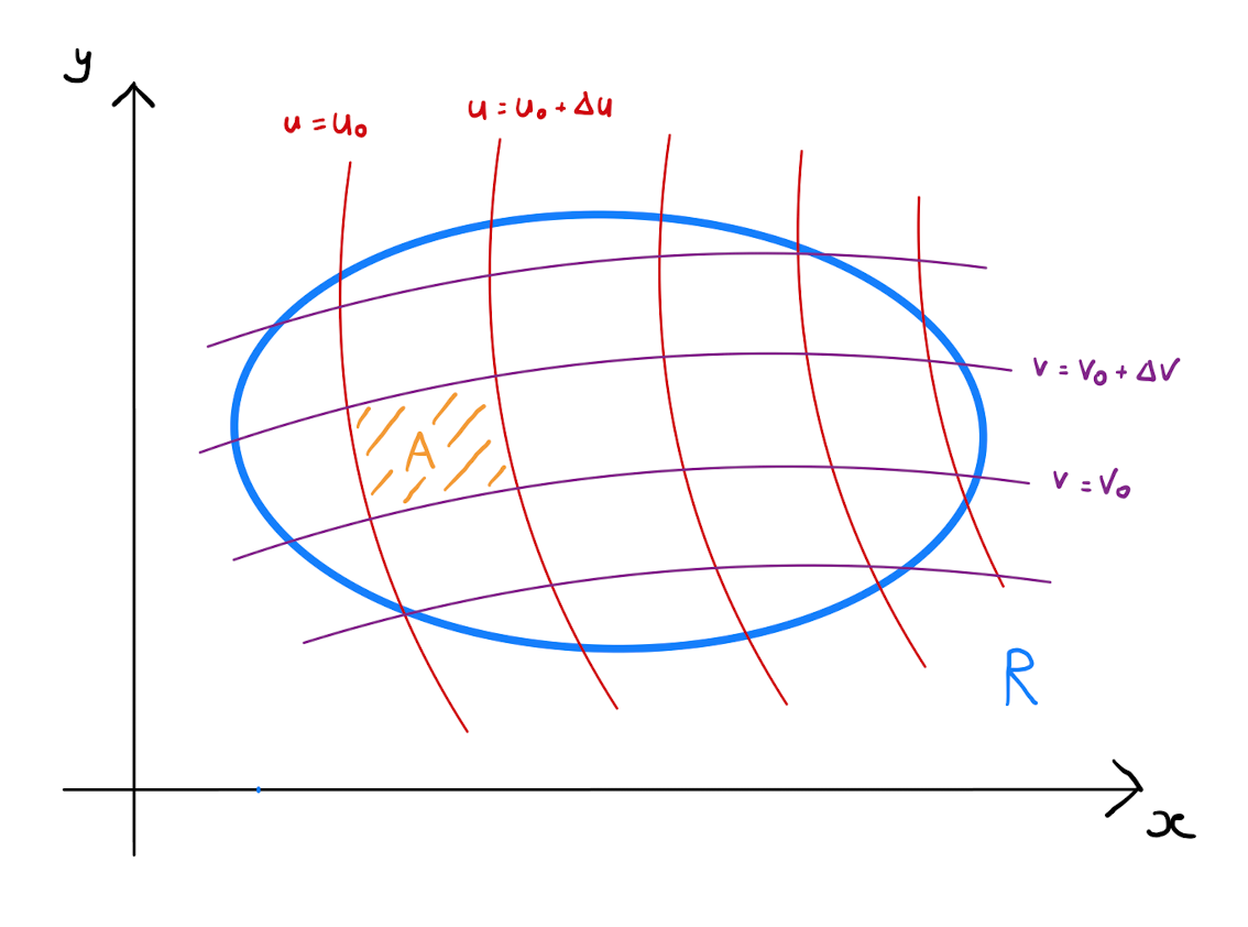
It follows that the integral \(I\) can be approximated by \[I \approx \sum\limits_{\text{copies of } A} f(x,y) \,\Delta A,\] where each \(f\) in the summation has been evaluated at a point within the appropriate copy of \(A\).

Since \(\Delta u\) and \(\Delta v\) are sufficiently small, it follows that \(A\) is approximately a parallelogram.

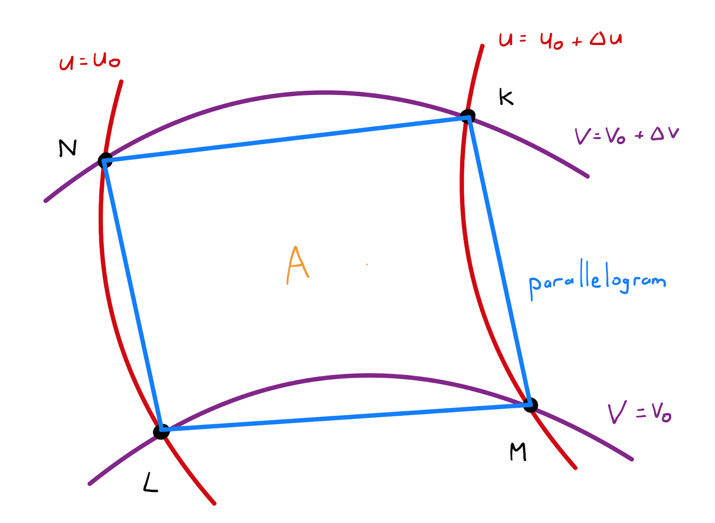
Formally, defining a parametrisation \(\mathbf{r}(u,v) = \left( x(u,v), y(u,v) \right)\), then the region \(A\) is approximated by the parallelogram with vertices:

\[\begin{align*} L &= \mathbf{r}(u_0,v_0), \\ M &= \mathbf{r}(u_0+ \Delta u,v_0), \\ N &= \mathbf{r}(u_0,v_0 + \Delta v), \\ K &= \mathbf{r}(u_0+ \Delta u,v_0 + \Delta v). \end{align*}\]

It follows that \[\Delta A \approx \left\lvert LM \times LN \right\rvert.\] By the theory of small changes seen in Section 5.1: \[LM = \mathbf{r}(u_0+ \Delta u,v_0) - \mathbf{r}(u_0,v_0) = \frac{\partial \mathbf{r}(u_0,v_0)}{\partial u} \Delta u,\] and similarly \[LN = \mathbf{r}(u_0,v_0 + \Delta v) - \mathbf{r}(u_0,v_0) = \frac{\partial \mathbf{r}(u_0,v_0)}{\partial v} \Delta v.\]

This allows us to write \(\Delta A\) in terms of \(\Delta u\) and \(\Delta v\):

\[\begin{align*} \Delta A &\approx \left\lvert \frac{\partial \mathbf{r}(u_0,v_0)}{\partial u} \Delta u \times \frac{\partial \mathbf{r}(u_0,v_0)}{\partial v} \Delta v \right\rvert \\[5pt] & = \left\lvert \frac{\partial \mathbf{r}(u_0,v_0)}{\partial u} \times \frac{\partial \mathbf{r}(u_0,v_0)}{\partial v} \right\rvert \Delta u \Delta v \\[5pt] & = \left\lvert \det \begin{pmatrix} \underline{\mathit{i}} & \underline{\mathit{j}} & \underline{\mathit{k}} \\ x_u & y_u & 0 \\ x_v & y_v & 0 \end{pmatrix} \right\rvert \Delta u \Delta v \\[5pt] &= \left\lvert \frac{\partial x}{\partial u} \frac{\partial y}{\partial v} - \frac{\partial x}{\partial v} \frac{\partial y}{\partial u} \right\rvert \Delta u \Delta v. \end{align*}\]

This motivates the following definition.

The Jacobian of a one-to-one transformation \(x=x(u,v), y=y(u,v)\), denoted \(\frac{\partial (x,y)}{\partial (u,v)}\), is given by \[\frac{\partial (x,y)}{\partial (u,v)} = \left\lvert \frac{\partial x}{\partial u} \frac{\partial y}{\partial v} - \frac{\partial x}{\partial v} \frac{\partial y}{\partial u} \right\rvert = \begin{vmatrix} \frac{\partial x}{\partial u} & \frac{\partial x}{\partial v} \\ \frac{\partial y}{\partial u} & \frac{\partial y}{\partial v} \end{vmatrix}.\]

Therefore \[\Delta A = \frac{\partial (x,y)}{\partial (u,v)} \,\Delta u \,\Delta v.\]

It follows that \[I \approx \sum\limits_{\text{rectangles}} f \big( x(u,v),y(u,v) \big) \frac{\partial (x,y)}{\partial (u,v)} \,\Delta u \,\Delta v,\] where the sum is over rectangles of width \(\Delta u\) and \(\Delta v\) filling \(S\) in the \((u,v)\)-plane, and each \(f\) in the summation has been evaluated at a point within the appropriate rectangle.

Taking the limit as \(\Delta u, \Delta v \rightarrow 0\), one obtains \[I = \int \int_{S} f \big( x(u,v),y(u,v) \big) \frac{\partial (x,y)}{\partial (u,v)} \,du \,dv.\]

In summary, all of the above is an informal proof of the following statement:

Suppose the region \(R\) in the \((x,y)\)-plane is mapped to the region \(S\) in the \((u,v)\)-plane by a one-to-one transformation \(x=x(u,v), y=y(u,v)\) where the first order partial derivatives of \(x\) and \(y\) are continous and the Jacobian \(\frac{\partial(x,y)}{\partial (u,v)}\) is only zero at isolated points of \(S\). If \(f(x,y)\) is a function with continuous partial derivatives on \(R\), then \[ \int \int_{R} f(x,y) \,dx \,dy = \int \int_{S} f \left( x(u,v), y(u,v) \right) \left\lvert \frac{\partial(x,y)}{\partial (u,v)} \right\rvert \,du \,dv.\]

Use the one-to-one transformation \(x(u,v)=\frac{1}{3} \left(v-u \right), y(u,v)= \frac{1}{3}\left( v+2u \right)\) to evaluate \(\int \int_{R} 2x+y \,dx \,dy\) for the finite region \(R\) bounded by the lines \(y=-2x+4\), \(y =-2x + 6\), \(y=x-2\) and \(y=x+1\).

Note \(f(x,y) = 2x+y\), so that \[f \big( x(u,v), y(u,v) \big) = 2 \cdot \frac{1}{3} \left(v-u \right) + \frac{1}{3}\left( v+2u \right)= v.\] Now looking at the bounding lines of \(R\), and rewriting them in terms of \(u\) and \(v\) by substitution, one obtains \[\begin{align*} y=-2x+4 \qquad &\text{becomes} \qquad v=4, \\[3pt] y=-2x+6 \qquad &\text{becomes} \qquad v=6, \\[3pt] y=x-2 \qquad &\text{becomes} \qquad u=-2, \\[3pt] y=x+1 \qquad &\text{becomes} \qquad u=1. \end{align*}\] It follows the region \(S\) is given as below:

Calculating the Jacobian, one obtains \[\frac{\partial(x,y)}{\partial (u,v)} = \begin{vmatrix} x_u & x_v \\ y_u & y_v \end{vmatrix} = \begin{vmatrix} -\frac{1}{3} & \frac{1}{3} \\ \frac{2}{3} & \frac{1}{3} \end{vmatrix} = - \frac{1}{3}.\] Therefore \[\begin{align*} \int \int_{R} 2x+y \,dx \,dy &= \int \int_{S} v \left\lvert -\frac{1}{3} \right\rvert \,du \,dv \\[3pt] &=\int_{4}^{6} \int_{-2}^{1} \frac{v}{3} \,du \,dv \\[3pt] &= \int_{4}^{6} \left[ \frac{uv}{3} \right]_{-2}^{1} \,dv \\[3pt] &= \int_{4}^{6} \frac{v}{3} - \left( - \frac{2v}{3} \right) \,dv \\[3pt] &= \int_{4}^{6} v \,dv \\[3pt] &= \left[ \frac{v^2}{2} \right]_{4}^{6} \\[3pt] &= 18 - 8 \\[3pt] &= 10. \end{align*}\]

12.3 Geometrical Interpretation of the Jacobian

Using the notation from the previous section, the small area \(\Delta A\) in \(R\) was the result of small changes \(\Delta u\) and \(\Delta v\) to \(u\) and \(v\), and therefore corresponds to a small area \(\Delta u \Delta v\) in \(S\). In particular:

\[\begin{align*} &\Delta A \approx \left\lvert \frac{\partial (x,y)}{\partial (u,v)} \right\rvert \Delta u \Delta v, \\[5pt] \implies \qquad &\left\lvert \frac{\partial (x,y)}{\partial (u,v)} \right\rvert \approx \frac{\Delta A}{\Delta u \Delta v}. \end{align*}\]

That is the Jacobian is the ratio of the two small corresponding areas. In other words at any point \((u,v) \in S\), the value \(\left\lvert \frac{\partial (x,y)}{\partial (u,v)} \right\rvert\) is the factor by which the area local to \((u,v)\) increases when mapped to \(R\).

Consider the one-to-one transformation from Theorem 2.1.1 to convert polar coordinates to Cartesian coordinates:

\[\begin{align*} x &= x (\rho,\varphi) = \rho \cos (\varphi), \\ y &= y (\rho,\varphi) = \rho \sin (\varphi). \end{align*}\]

Calculate the Jacobian of this transformation as

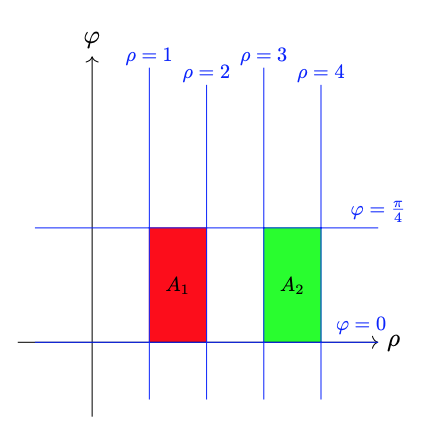
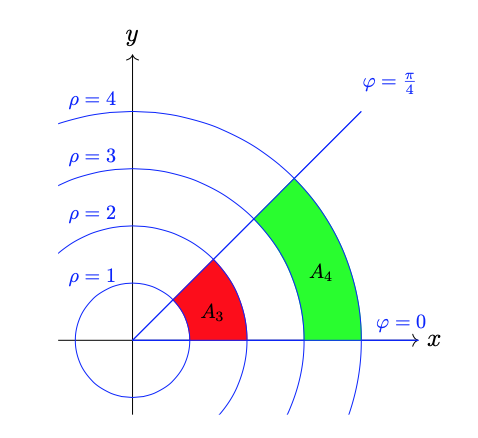
\[\frac{\partial (x,y)}{\partial (\rho,\varphi)} = \begin{vmatrix} x_{\rho} & x_{\varphi} \\ y_{\rho} & y_{\varphi} \\ \end{vmatrix} = \begin{vmatrix} \cos (\varphi) & -\rho \sin(\varphi) \\ \sin(\varphi) & \rho \cos(\varphi) \end{vmatrix} = \rho \cos^{2}(\varphi) + \rho \sin^{2}(\varphi) = \rho.\]

Consider the regions \(A_{1},A_{2}\) in the \((\rho,\varphi)\)-plane, and the regions \(A_{3},A_{4}\) in the \((x,y)\)-plane, as depicted:

Via standard area calculations, obtain

\[\begin{align*} \text{Area}(A_{1}) &= \frac{\pi}{4} \\ \text{Area}(A_{2}) &= \frac{\pi}{4} \\ \text{Area}(A_{3}) &= \frac{3 \pi}{8} \\ \text{Area}(A_{4}) &= \frac{7 \pi}{8} \end{align*}\]

Note \(A_{3}\) is the image of \(A_{1}\) under the polar coordinate transformation. Consider the ratio of \(A_{3}\) to \(A_{1}\): \[\frac{A_{3}}{A_{1}} = \frac{\frac{3 \pi}{8}}{\frac{\pi}{4}} = \frac{3}{2}.\] The value \(\frac{3}{2}\) is the average value taken by the Jacobian \(\frac{\partial(x,y)}{\partial(\rho, \varphi)} =\rho\) over the region \(A_{1}\).

Also note \(A_{4}\) is the image of \(A_{2}\) under the polar coordinate transformation. Consider the ratio of \(A_{4}\) to \(A_{2}\): \[\frac{A_{4}}{A_{2}} = \frac{\frac{7 \pi}{8}}{\frac{\pi}{4}} = \frac{7}{2}.\] The value \(\frac{7}{2}\) is the average value taken by the Jacobian \(\frac{\partial(x,y)}{\partial(\rho, \varphi)} =\rho\) over the region \(A_{2}\).

12.4 Jacobian of the Inverse

It is known that given a univariate function \(z=z(t)\), that \(\frac{dt}{dz} = \frac{1}{\left( \frac{dz}{dt} \right)}\) provided \(\frac{dz}{dt} \neq 0\). However for the multivariate one-to-one transformation \(x=x(u,v), y=y(u,v)\), it is not necessarily true that \(\frac{\partial u}{\partial x} = \frac{1}{\left( \frac{\partial x}{\partial u} \right)}\).

The two-dimensional analogue of the identity in the univariate case is a relationship between the Jacobian of an inverse transformation in terms of the Jacobian of the original transformation.

Let \(x=x(u,v), y=y(u,v)\) be a one-to-one transformation such that \(\frac{\partial (x,y)}{\partial(u,v)} \neq 0\). Then the Jacobian of the inverse transformation \(u=u(x,y), v=v(x,y)\) is given by \[\frac{\partial (u,v)}{\partial(x,y)} = \frac{1}{\left( \frac{\partial (x,y)}{\partial(u,v)} \right)}.\]

Often an application of Lemma 12.4.1 can present an easier method to calculate the Jacobian of a transformation than direct computation does.

Consider the transformation

\[\begin{align*} \rho &= \rho (x,y) = \sqrt{x^2 + y^2}, \\ \varphi &= \varphi(x,y) = \arctan \left( \frac{y}{x} \right). \end{align*}\]

Calculate the Jacobian of the transformation.

The transformation is recognised as the transformation to convert from Cartesian coordinates to polar coordinates. In particular it the inverse of the transformation to convert polar coordinates to Cartesian coordinates given by

\[\begin{align*} x &= x (\rho,\varphi) = \rho \cos (\varphi), \\ y &= y (\rho,\varphi) = \rho \sin (\varphi). \end{align*}\]

We saw in Example 14.3.1 that \(\frac{\partial (x,y)}{\partial (\rho,\varphi)} = \rho\). Hence

\[\frac{\partial (\rho,\varphi)}{\partial (x,y)} = \frac{1}{\left( \frac{\partial (x,y)}{\partial (\rho,\varphi)}\right)} = \frac{1}{r}.\]