MATH1006 Calculus
2023-05-22
Chapter 1 Functions of Several Variables
1.1 Recap of Functions of One Variable
The Autumn semester of MATH1006 Calculus centered on the study of functions of one real variable. Such functions are known as univariate functions, that is, they take one variable as input.
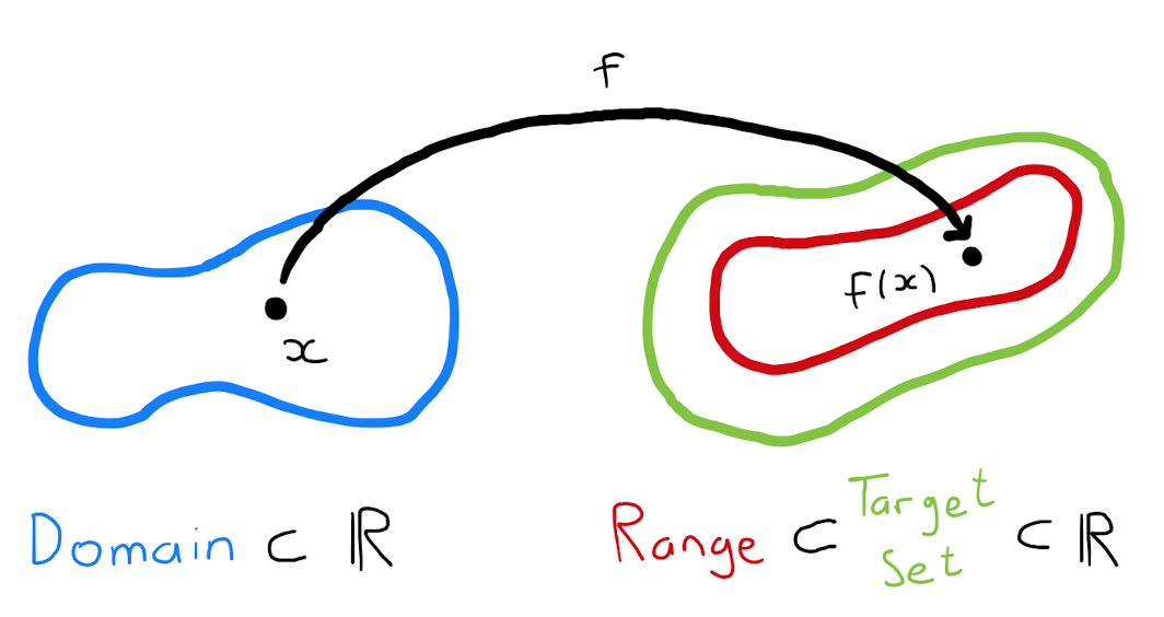
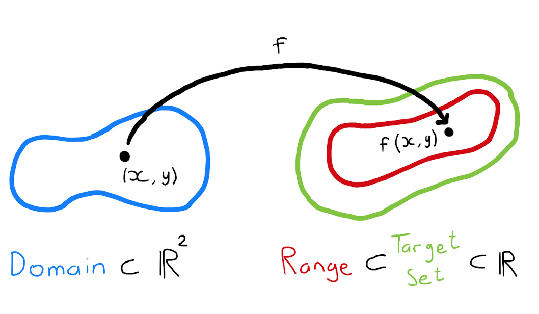
A univariate function of real variables, denoted \[\begin{align*} f: X &\longrightarrow Y \\ x &\longmapsto y = f(x) \end{align*}\] is a rule that assigns to each element in \(X\) exactly one element in \(Y\), where \(X \subseteq \mathbb{R}\) and \(Y \subseteq \mathbb{R}\).
With regards to Definition 1.1.1, we have the further additional terminology:
The variable \(x\) is called the independent variable;
The variable \(y\) is called the dependent variable;
The set \(X\) is called the domain of the function;
The set \(Y\) is called the target set of the function;
The set \(\left\{ f(x) : x \in X \right\}\) is called the image or the range of the function.
Note that the range of a function is a subset of the target set \(Y\). It is possible that these two sets are equal but this is not necessarily true.
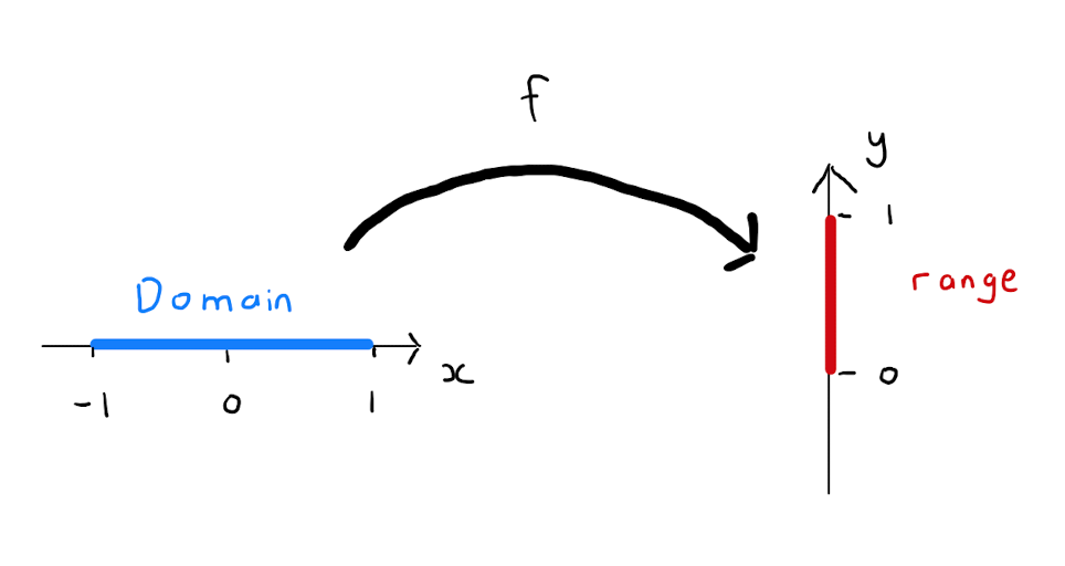
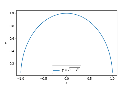
Consider the set \(X = [-1,1] \subset \mathbb{R}\). Define the function \[\begin{align} f: X &\longrightarrow \mathbb{R}, \\ f(x) &= \sqrt{1 - x^2}. \end{align}\] The domain of \(f\) is given by \([-1,1]\). The target set of \(f\) is \(\mathbb{R}\). The range of \(f\) is \([0,1]\).
A univariate function of real variables can be represented graphically in two dimensions. The set of points \(\left\{ (x,y) : y = f(x) \right\}\) is a curve that represents the function \(f\), known as the graph of the function.
Further examples of univariate function can be found in the Autumn semester lecture notes.
1.2 Multivariate Functions
The focus of MATH1006 Calculus throughout the Spring semester will be so-called multivariate functions, that is functions with more than one input variable, rather than univariate functions. Topics such as derivatives and stationary points will be again be studied, only now in this new, more general setting.
A multivariate function of real variables, denoted \[\begin{align*} f: X &\longrightarrow Y \\ x = (x_1, \ldots, x_n) &\longmapsto y = f(x_1,x_2, \ldots, x_n) \end{align*}\] is a rule that assigns to each element in \(X\) exactly one element in \(Y\), where \(X \subseteq \mathbb{R}^{n}\) and \(Y \subseteq \mathbb{R}\) with \(n \in \mathbb{Z}_{>1}\).
The crucial aspect of the definition is that there are multiple independent variables. A perturbation to any of these independent variables may cause some change to the dependent variable.
The terminology domain, target set and range are still used to discuss multivariate functions.
Consider a solid cone with height \(h\) and radius \(r\):

It is well known that the volume of the cone is given by \(V= \frac{\pi}{3} r^2 h\). Indeed one can think of \(V\) as a function \(V(r,h)\) of the independent variables \(r\) and \(h\). If the height of the cone increases, then the volume \(V\) will increase, even if the radius remains constant throughout. Likewise any change in the radius \(r\) will result in a change in \(V\), even if the height is unchanged.
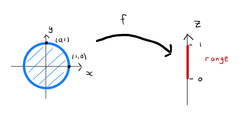
Consider the set \(X = \left\{ (x,y) : x^2 + y^2 \leq 1 \right\} \subset \mathbb{R}^{2}\). Define the multivariate function of two variables given by
\[\begin{align}
f: X &\longrightarrow \mathbb{R}, \\
f(x,y) &= \sqrt{1 - x^2 - y^2}.
\end{align}\]
The domain of \(f\) is given by \(\left\{ (x,y) : x^2 + y^2 \leq 1 \right\}\). The target set of \(f\) is \(\mathbb{R}\), and the range of \(f\) is \([0,1]\).
Stoke’s Law describes the friction or drag \(D\) on a sphere of radius \(r\) that moves through a liquid of viscosity \(v\) at a speed \(s\). Specifically \[D= 6 \pi rvs.\]
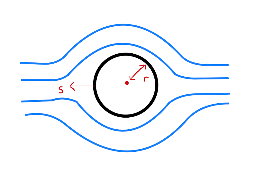
One can think of \(D\) as a function \(V(r,v,s)\) of \(r,v,s\). That is, \(D\) is the dependent variable, and there are three independent variables \(r\), \(v\) and \(s\).
1.3 Graphical Representation of a Function of Two Variables
Consider a function \(z=f(x,y)\) of two independent variables. Then \(f\) can be represented graphically, as was the case for univariate functions. However, now we have three variables: the independent \(x, y\), and the dependent \(z\). Hence the function will require three dimensions to represent in a plot. Typically one uses the standard Cartesian \(x,y,z\) coordinate system in \(\mathbb{R}^{3}\)
Given a function of two real variables \(f\), the set \(\left\{ (x,y,z) : z = f(x,y) \right\} \subset \mathbb{R}^{3}\) is the surface representing \(f\).
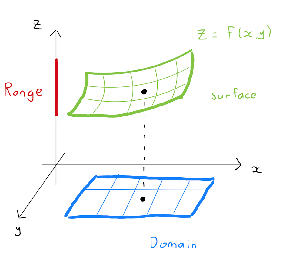
Each point \((x_0, y_0)\) in the domain of \(f\), uniquely corresponds to a point \(\left( x_0,y_0, f(x_0,y_0)\right)\) on the surface.
Sketching surfaces by hand is often difficult. Using computer software is often the best way to visualise these surfaces.
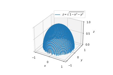
Recall the function \(z = f(x,y) = \sqrt{1 - x^2 - y^2}\) of two real variables from Example 1.2.3. The surface of \(f\) is a hemisphere as shown below.
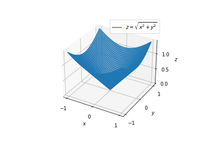
The surface of the function \(z = f(x,y) = \sqrt{x^2 + y^2}\) is a circular cone:
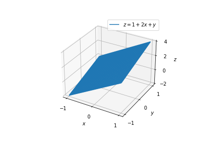
The surface of the function \(z = f(x,y) = a+bx+cy\) where \(a,b,c\) are constants with \((b,c) \neq (0,0)\), is a plane:
1.4 Level Curves
An alternative solution to the difficulty in sketching surfaces in three dimensions is to plot level curves.
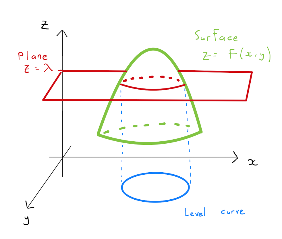
Let \(z=f(x,y)\) be a function of two variables. The level curve of \(f\) at height \(\lambda\) is the set of points defining a curve in \(\mathbb{R}^{2}\), given by \[\left\{ (x,y) \in \mathbb{R}^{2} : f(x,y) = \lambda \right\}.\]
Specifically consider the surface corresponding to the function \(f\). Orientate the three-dimensional space so that the \(z\)-axis is vertical. One can look at all the points on the surface at a height \(\lambda\) above the horizontal \((x,y)\)-plane. These are the points on the surface that also lie on the plane \(z=\lambda\). The preimage of this collection of points under \(f\) is the level curve of \(f\) at height \(\lambda\).
Level curves are actually a concept we are already familiar with: think of contour lines on a map of a hill. A contour line labelled \(1000\) is a curve marking all the points that \(1000\) meters above see level. That is if we could model the hill using a function \(f\), the level curve of \(f\) at height \(1000\) would be our contour line.
Level curves are also commonly referred to as contour plots.
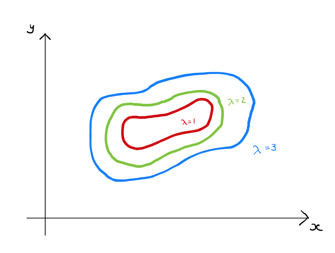
By plotting in \(\mathbb{R}^{2}\) the level curves of a function \(f\) at a collection of heights helps us to visualise the surface of \(f\) to some extent. This is identical fashion to how the contour lines on a map inform us of the steepness and shape of a hill.
Recall the function \(z = f(x,y) = \sqrt{x^2 + y^2}\) from Example 1.3.3, whose surface is a circlular cone. Then the level curve of \(f\) at height \(\lambda\) is the set of points \((x,y)\) that satisfy:
\[\begin{align*}
\sqrt{x^2 + y^2} &= \lambda \\
\iff \qquad x^2 + y^2 &= \lambda^2,
\end{align*}\]
which we know to describe the circle of radius \(\lambda\) centered at the origin for positive values of \(\lambda\). It is straightforward to plot a number of level curves in \(\mathbb{R}^2\). It is worth noting that the level curve of \(f\) at height \(\lambda<0\) is the empty set.
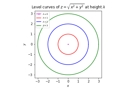
Observe that as \(\lambda\) increases linearly from \(0\), so does the radius of the level curve.
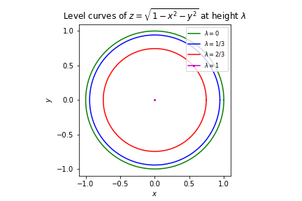
Recall the function \(z = f(x,y) = \sqrt{1-x^2 - y^2}\) from Example 1.3.2, the surface of which is a hemisphere. Calculate that the level curve of \(f\) at height \(\lambda>0\) is the set of points \((x,y)\) satisfying
\[\begin{align*}
\sqrt{1-x^2 - y^2} &= \lambda \\
\iff \qquad 1 - x^2 - y^2 &= \lambda^2 \\
\iff \qquad x^2 + y^2 &= 1 - \lambda^2.
\end{align*}\]
For \(\lambda>1\), the level curve will be the empty set. For \(0 \leq \lambda \leq 1\), the level curve will be the circle of radius \(\sqrt{1-\lambda^2}\) centered at the origin. It is worth noting that the closer level curves indicate a steeper surface. Since \(f\) was defined specifically using the positive square root, there are no points \((x,y)\) such that \(f(x,y)<0\). Therefore the level curves of \(f\) at negative heights are the empty set.
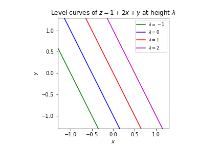
Consider the function \(z = f(x,y) = a+bx+cy\) in Example 1.3.4 describing a plane. The level curves of \(f\) at a collection of incrementing heights, are both parallel and equally spaced. This is because the surface has constant slope everywhere.
1.5 Graphical Representation of a Function of Three Variables
Consider a function \(u=f(x,y,z)\) of three independent variables. If we wanted to represent \(f\) graphically, we would need to plot a shape in four dimensions, one for each of the coordinates \(u,x,y,z\). This is simply not feasible.
One work around is to plot a number of surfaces in three dimensions to study cross-sections of the four-dimensional shapes. This is achieved by fixing one of the variables \(x,y,z\) to a collection of suitably chosen constants.
Alternatively one can plot the level surfaces of \(f\).
Let \(u=f(x,y,z)\) be a function of three variables. The level surface of \(f\) at height \(\lambda\) is the set of points defining a surface in \(\mathbb{R}^{3}\), given by \[\left\{ (x,y,z) \in \mathbb{R}^{3} : f(x,y,z) = \lambda \right\}.\]
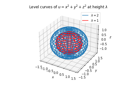
Consider the function \(u = f(x,y,z) = x^2+y^2+z^2\). The level surface of \(f\) at height \(\lambda\) is the set of points \((x,y,z)\) that satisfy:
\[x^2 + y^2+z^2 = \lambda,\]
that is, a sphere of radius \(\sqrt{\lambda}\) centered at the origin for positive values of \(\lambda\).