7.1 Supplemental methods
7.1.1 Calibrated parameters
Two model parameters were calibrated: The average number of components transfused to each recipient and the number of components transfused per collected donation. Data from the 2015 National Blood Collection and Utilization Survey (NBCUS) were used for calibration [34]. The average number of components produced per donation (1.421) was calculated as the total number of Red Blood Cells, Platelets, and Plasma transfused to recipients (17.9 million) divided by the total number of whole blood and red blood cell donations collected (12.6 million), as estimated in NBCUS. The components transfused per recipient (3.578) was estimated as the total number of Red Blood Cells, Platelets, and Plasma components transfused to recipients from NBCUS (17.9 million) divided by the estimated total number of recipients (5 million) estimated from Ellingson 2017 [34]. These parameters were not varied in sensitivity analysis.
7.1.2 Input parameters
All input parameters are in Tables 2.1, 7.1, 7.2, or 7.3. Modeling assumptions associated with input parameters include:
Number of recipients
Total, 50 states: The 50 states and D.C. number of recipients in a year was estimated at 5 million based on the often-cited 2007 National Blood Collection and Utilization Survey.2 While this estimate was originally for RBCs only, the decline in transfusion utilization in years since1 suggests that today this estimate is appropriate to use for recipients of all components rather than RBCs alone.
Puerto Rico: For Puerto Rico, ID-NAT testing data indicated that 78,046 donations had been collected in the first 52 weeks after full implementation of ID-NAT. By assuming Puerto Rico had the same ratio of donations collected to recipients transfused as the 50 states (2.52), we derived the estimate of 31,000 Puerto Rican transfusion recipients. We assumed 50% received blood collected during the high mosquito season and 50% received blood during the low mosquito season.
Component-specific transfusion-transmissibility estimates: As shown in Table 2.1 of the main text, we assumed that a ZIKV-infectious RBC or PLT component has a 50% chance of leading to TTZ, and a ZIKV-infectious FFP component has a 90% chance of leading to TTZ. These are estimates that the authors consider to be conservative (i.e. unlikely to underestimates of the infectiousness of a ZIKV-infectious component). Studies of compartments with ZIKV viremia have been conducted, but infectivity studies are very challenging to complete. We are now conducting infectivity studies in the Macaque model that include escalating dose IV inoculations with ZIKV RNA+ plasma derived from FFP components from donors detected in pre-IgM/IgG and post-IgM/IgG stages of infection, as well as with RBC derived from LR pRBC components from donations that tested very low-level reactive by ID-NAT but had substantial levels of ZIKV RNA associated with RBC samples. These studies, which are in progress, will provide additional data to support our inference that the risk of TT is primarily associated with components derived from RNA+/IgM- donations, as well as the relationships between ZIKV VL in those donations and infectivity titers.
MP-NAT clinical sensitivity: The clinical sensitivity was estimated based on 200 ID-NAT confirmed RNA reactive donations interdicted in Puerto Rice that were IgM negative. We focused on IgM negative donations alone because the evidence suggests IgM positive donations are most likely not infectious and we did not want to artificially understate the clinically meaningful sensitivity of MP-NAT. Notably, this is in contrast to our decision to consider RNA positive donations infectious in determining the ZIKV infectious rate in donations without regard to IgM reactivity, which was made to ensure we did not underestimate the rate of ZIKV infectiousness in donations. Of these 200 donations, 14 were not reactive in simulated mini-pools achieved through dilutional testing, leading to our MP-NAT sensitivity estimate of 92.5%.
Productivity and consumption: We assumed recipients and partners lost productivity for each day of illness equal to the 2016 median total money income by age. For premature death, we subtracted the 2016 mean consumption by age group from the 2016 mean total dollar income and summed for the years of life lost. For infants born with congenital Zika syndrome, regardless of whether the pregnancy resulted in a stillbirth or live birth, we included productivity loss netted consumption for an entire lifetime of earning at average life expectancy in the costs.
Continuous time discounting: We assumed a discount factor of 0.03 per year discounted continuously. Any cost or QALY outcome that was experienced over a period from ta to tb expressed in years from transfusion were multiplied by a discount factor γ calculated as:
\[ \gamma (t_a,t_b) = \frac{1-e^{-0.03(t_b-t_a)}}{0.03(t_b-t_a)} \]
Medical costs of birth: Our simulation only totaled costs and QALYs lost due to transfusion-transmission of Zika. Thus, if no congenital Zika syndrome (CZS) occurred, the costs associated with a pregnant recipient or sexual partner were 0. If the infant was infected with CZS, the medical cost of a healthy birth was subtracted from the medical cost of a birth with CZS (or the cost of a stillbirth). Due to this approach, the net medical costs of infants who were stillborn due to CZS were negative. However, the lifetime productivity costs associated with a stillbirth due to CZS far outweighed the small negative medical costs.
False-positive and true-positive costs: We assume that initially-reactive donations are removed from the blood supply regardless as to whether confirmatory testing suggests the donations were false-positive. The cost is meant to encompass the cost of confirmatory testing, the cost of destroying the donation, and the cost of counseling the donor regarding their test result. We did not include the potential stress or unnecessary medical costs experienced by donors whose blood tested false-positive, nor the potential medical costs or health benefits conferred to the donor by notification of a true-positive test result.
7.1.3 Structure overview
We developed a microsimulation with the following components.
Repetitions: The number of repetitions completed for each donor group corresponded to the number of recipients in each group per year as reported in Table 2.1. A repetition consisted of the following three main steps:
Sampling a recipient: We used a dataset from SCANDAT (Scandinavian Donations and Transfusions)3 that contained the age, sex, and number of components of platelets, plasma, and red blood cells received by transfusion recipients, adjusted by a multiplier that ensured the mean components-per-recipient matched that of U.S. recipients found in NBCUS. In each repetition, we randomly selected a recipient from this database. The baseline survival of the recipient was then drawn from a survival distribution that was determined following the process described in a later section.
Determining the probability of transfusion-transmission of Zika: For each recipient, the probability they experienced a transfusion-transmission under each strategy was calculated based on: (1) the number of components received of each type, (3) the assumed transfusion-transmissibility of each component, (2) the ZIKV infectious donation rate corresponding to the recipient group, (3) the sensitivity and specificity of the test used specifically for the given donor group under the given policy. Specifically, the probability of transfusion-transmission was calculated as:
\[ P_T = 1 - P_{T \mid RBC+} (1 - P^{n_{RBC}}_{Z-}) \times P_{T \mid PLT+} (1 - P^{n_{PLT}}_{Z-}) \times P_{T \mid FFP+} (1 - P^{n_{FFP}}_{Z-}) \]
Where \(P_T\) is the probability of transfusion-transmission; \(P_{T|RBC+}\) (respectively, \(P_{T|PLT+}\) and \(_{PT|FFP+}\)) is the probability of transmission given that a ZIKV infectious RBC component (respectively, PLT and FFP) has been transfused; \(n_{RBC}\) (respectively, \(n_{PLT}\) and \(n+{FFP}\)) is the number of RBC components transfused to the recipient (respectively PLT and FFP components); and \(P_{z-}\) is the probability that each component is not ZIKV infectious, defined as one minus the ZIKV infectious rate for the donor group.
- Determining the health and economic outcomes: Once \(P_Z\) is calculated, all outcomes are calculated according to the decision tree in Figure 7.1 using the conditional Monte Carlo efficiency improvement described below. Aggregated outcomes included ZIKV transfusion transmissions, total costs, blood center costs, productivity costs, recipient medical costs, partner medical costs, infant medical costs, partner’s infant’s medical costs, true positive donations interdicted, false positive donations interdicted, congenital Zika syndrome cases, Guillain-Barre syndrome cases, mild febrile illness cases.
Iterations: Each iteration generated as many samples from each donor group as would be transfused in a year. To develop stable estimates, the base case results were based on 100 iterations for the 50 states and 3,000 samples for Puerto Rico. In probabilistic sensitivity analysis, one iteration was completed for 10,000 unique draws of the input parameters from distributions. To ensure Puerto Rico results were stable estimates, we ran 100 times as many repetitions in each PSA iteration as were run in a single base-case iteration.
7.1.4 Sampling recipients
Sex and age group (in 5-year blocks of 0, 5, … , 85, 90) were sampled directly from the SCANDAT data. The recipient’s exact integer age is chosen uniformly at random (e.g. for age group 65, an age of 65, 66, 67, 68, or 69 is assigned). For recipients in the 90+ age group, we choose an age between 90 and 94, even though recipients could be older. Based on the National Blood Collection and Utilization survey, we determined that the average American recipient receives 3.58 components, while the average recipient in the SCANDAT dataset received 8.75 components. To better approximate recipients in the United States, we divided the number of components received by each recipient by 0.41. Post-Transfusion Survival: A precise post-transfusion survival in years was calculated by sampling from a discrete distribution that represents the probability the recipient lived i whole years post-transfusion, calculated as described below. To account for the fact that the recipient may die at any point during the following year, a random number between 0 and 1 is then added to this integer.
The i-year survival probability \(\hat{r}_{i,j,k}\) is the probability a recipient lives beyond the ith whole year following the transfusion episode. k indicates the recipient’s age at transfusion and j indicates the recipient class (binned by age-group, RBC components received, PLT components received, and FFP components received). \({\hat{r}}_{i,j,k}\) is calculated as follows:
\[ \hat{r}_{i \in \{0,...,4\},j,k} = r_{i,j} + \frac{b_j}{\max_j b_j} (h_{k,i} - r_{i,j}) \\ \hat{r}_{i \in \{5,...,100-k\},j,k} = \hat{r}_{i-1, j,k} (1-p_k)\\ \hat{r}_{i = 101-k,j,k} = 0 \]
The term \(r_{i,j}\) refers to the unadjusted \(i\)-year survival for the age bin indicated by recipient class \(j\), from Kleinman 2004 [81] (used for first 5 years post-transfusion only). \(h_{i,j}\) refers to the mean survival for Americans of a given age, derived from 2014 U.S. Life Tables5, described below. The term \(b_j\) is a multiplier derived from the SCANDAT dataset specific to bin \(j\), described below. \(h_{i,j}\) is calculated as follows:
$$ h_k=1-p_k i=0\ h_k = h_{k-1} (1-p_k) i>0
$$ where \(p_k\) is the probability of all-cause mortality between ages \(k\) and \(k+1\) from CDC life tables. The multiplier \(b_j\) is calculated as follows:
\[ b_i=\frac{c_j-\bar{c_j}}{\bar{c_j}} \]
Where \(c_j\) is the mean observed post-transfusion life years per recipient for a given age-component bin, and \(\bar{c_j}\) is the mean post-transfusion life years per recipient for all bins in that age group. The term \(c_j\) is calculated to include both recipients whose deaths were observed and recipients who were censored, under the rationale that censorship is random across bins and the bins are sufficiently large (>390 recipients per bin).
7.1.5 Conditional Monte Carlo Approach
Under a traditional Monte Carlo approach, a small minority of recipients would experience transfusion-transmission of Zika, and it we would expect it to take several million iterations to observe even a handful of rare Zika sequelae such as Guillain-Barre syndrome and congenital Zika syndrome. To address this, we calculated outcomes for every repetition assuming transfusion-transmission occurred and then used conditional probabilities to estimate the expected outcome: \[ E(O)= P_ZO_Z + (1-P_Z)O_{¬Z} \] Where \(E(O)\) is the expected outcome; \(P_Z\) is the probability of transfusion-transmission of Zika as described earlier; \(O_Z\) is the simulated outcome assuming transfusion-transmission of Zika occurred; and \(O_{¬Z}\) is the simulated outcome assuming no transfusion-transmission of Zika. Because blood center costs and donations interdicted as true positives or false positives do not change depending on whether transfusion-transmission occurs, these outcomes were calculated in the traditional way. For all other outcomes, however, \(O_{¬Z}\) is 0 with probability 1. Thus, we could exclude the second term, giving the simpler equation:
\[ E(O)= P_Z O_Z \]
7.1.6 Defining Areas Experiencing Known Local Transmission for Location- and Travel-Based Screening Policies
Domestic areas: Two areas within the 50 states were designated by the CDC as experiencing local mosquito transmission for some portion of the period of our analysis.6 Out of an abundance of caution, we defined the areas that would undergo heightened screening under our location- and travel-based policies as larger than the areas the CDC identified, as the maps in Figures 7.2 and 7.3 show. We defined the period in which heightened screening measures would be applied as December 14, 2016 – August 29, 2017 for the Texas gulf coast and as August 1, 2016 – June 2, 2017 for south Florida. Below are the areas included in those experiencing a local transmission for the traveler-adapted strategy:
South Florida: Fort Myers-Cape Coral, FL MSA, Miami, FL PMSA, Fort Lauderdale, FL PMSA, West Palm Beach-Boca Raton, FL MSA, FLORIDA REMAINDER OF STATE, FLORIDA UNSPECIFIED
Texas Gulf Coast: McAllen-Edinburg-Mission, TX MSA, Corpus Christi, TX MSA, Beaumont-Port Arthur, TX MSA, TEXAS REMAINDER OF STATE, TEXAS UNSPECIFIED
International areas: For the travel-based policies, screening was heightened for any donor who discloses travel to one of the two domestic areas of local transmission during the period of transmission or to a foreign country with local transmission. Our list of foreign countries was based on a list in the CDC website [61] and included:
- AFRICA, ANGUILLA, ANTIGUA & BARBUDA, ANTILLES, ARGENTINA, ARUBA, BARBADOS, BELIZE, BOLIVIA, BRAZIL, BRITISH VIRGIN ISLANDS, CAMBODIA, CARIBBEAN, CENTRAL AMERICA, COLOMBIA, COSTA RICA, CUBA, DOMINICA, DOMINICAN REPUBLIC, ECUADOR, EL SALVADOR, FIJI, GHANA, GRENADA, GUATEMALA, HAITI, HONDURAS, INDIA, INDONESIA, JAMAICA, KENYA, MALAYSIA, MEXICO, MONTSERRAT, NICARAGUA, NIGERIA, PANAMA, PAPUA NEW GUINEA, PARAGUAY, PERU, PHILIPPINES, PUERTO RICO, SINGAPORE, SOUTH AMERICA, ST VINCENT & THE GRENADINES, THAILAND, TRINIDAD & TOBAGO, TURKS & CAICOS ISLANDS, US VIRGIN ISLANDS, VENEZUELA, VIETNAM, WEST INDIES, WINDWARD ISLANDS, PAKISTAN, SAN JUAN (SJU), BANGLADESH, BURMA, CAPE VERDE, CENTRAL AFRICAN REPUBLIC, GABON, GUINEA, GUYANA, LAOS, MALI, SAN JUAN (NEW), SENEGAL, ST KITTS-NEVIS, ST LUCIA, SUDAN, TANZANIA, UGANDA, UZBEKISTAN, WESTERN SAMOA
Travel: From the 1995 American Travel Survey data [66], we determined the proportion of U.S. residents who had traveled to a foreign country with local Zika transmission (2.64%). We determined the proportion of residents with travel to a domestic area that experienced local transmission (2.6% for TX; 3.9% for FL). We then multiplied by the proportion of the year that local transmission was occurring (75% for TX; 91.6% for FL) and summed with the proportion of residents with international travel to a country with local transmission to get the total proportion of residents with travel to an area experiencing local transmission (8.13%). We assumed blood donors did not differ from typical U.S. residents in the proportion with travel to an area of Zika local transmission.
7.1.7 Linear regression meta-modeling of PSA data
Each PSA iteration produced a vector of input parameters drawn from independent distributions and several outcomes. First, Input variables were standardized to have a mean of 0 and a standard deviation of 1 with the following equation:
\[ z_{ij}=\ \frac{x_{ij}-\bar{x_j}}{{\bar{\sigma}}_j} \]
Where \(x_{ij}\) is the ith observation of parameter \(j\); \(\bar{x_j}\) is the sample mean of parameter \(j\); and \(\ {\bar{\sigma}}_j\) is the sample standard deviation of parameter \(j\).
Then, we built a series of linear regression models using all input variables as predictors for one outcome at a time. The coefficients and corresponding p-values were recorded for each model. We then applied the Benjamini-Yekutieli adjustment to the p-values [151]. For coefficient \(\beta_j\ \) with a significant p-value, we can interprete the coefficients as follows: A 1 standard deviation increase in parameter \(x_j\) is associated with a \(\beta_j\) increase in outcome \(y\), ceteris paribus.
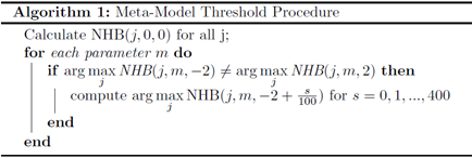
We then use our meta-models to determine whether the preferred strategy is sensitive to a univariate change in a parameter value up to ±2 standard deviations. To do so, we calculate net health benefit for policy \(j\) with parameter \(m\) increased by \(i\) standard deviations:
\[ NHB(j,0,0) = \beta_{j,0} - \frac{\alpha_{j,0}}{\lambda}\\ NHB(j,m,i) = \beta_{j,0} + i \beta_{j,m} - \frac{\alpha_{j,0} + i \alpha_{j,m}}{\lambda} = NHB(j,0,0) + i \Big( \beta_{j,m} - \frac{ \alpha_{j,m}}{\lambda} \Big) \]
Where \(\beta_{j,m}\) is the linear regression coefficient for parameter m from the linear regression predicting QALYs under policy \(j\), and \(\alpha_{j,m}\) is the linear regression coefficient for parameter \(m\) from the linear regression predicting cost under policy \(j\). \(\lambda\) is the willingness-to-pay threshold expressed as dollars per QALY. Using these equations and the following algorithm, we determine whether the optimal policy varies as the input parameters are varied over the range 0±2\({\bar{\sigma}}_j\) one at a time: