Chapter 4 Seurat QC Cell-level Filtering

library(Seurat)
library(data.table)
library(tidyverse)
library(magrittr)
library(gridExtra)

4.1 Description

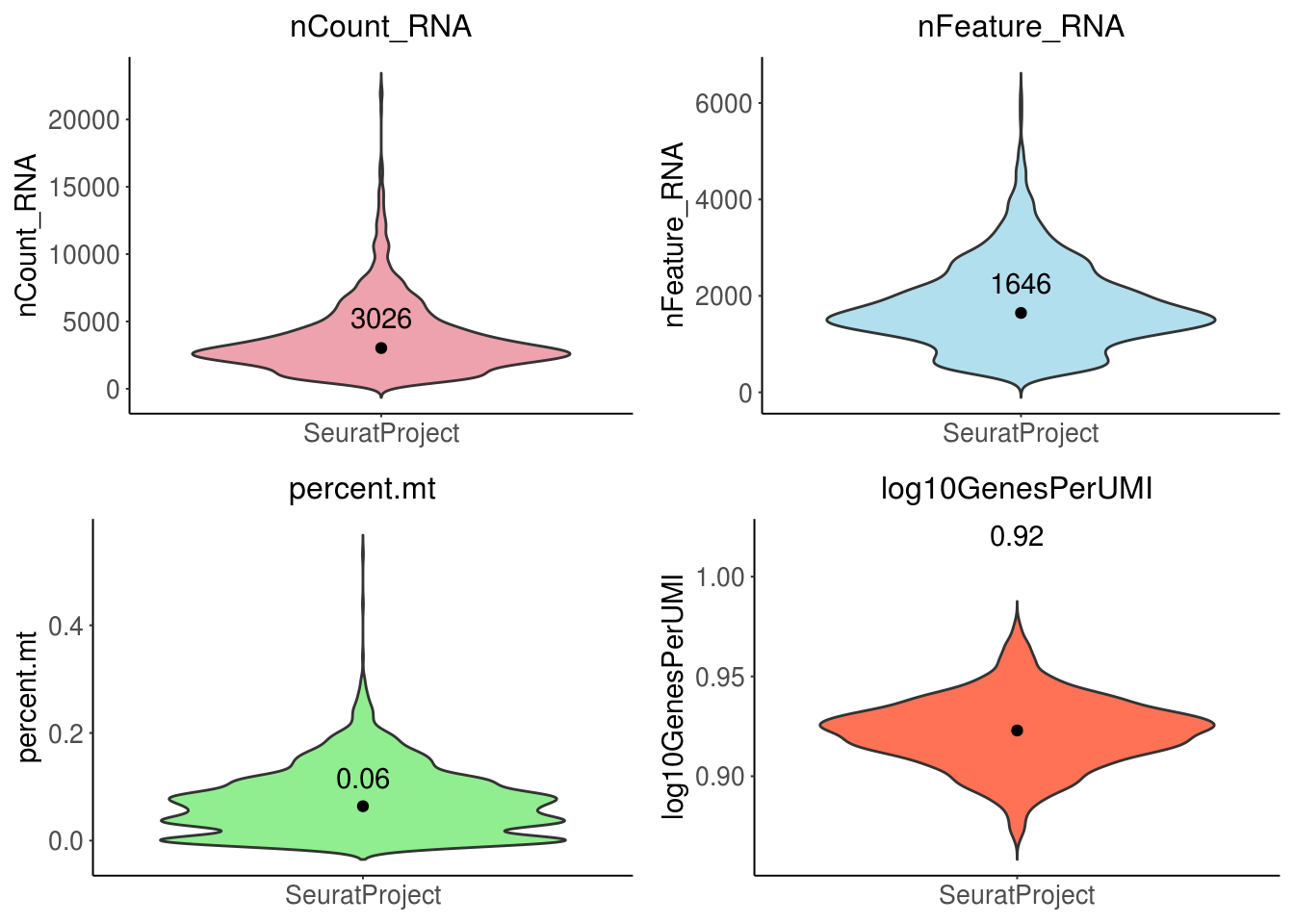
Basic quality control for snRNA-seq: check the distribution of

• number of UMIs per cell

  • should above 500

• number of genes detected per cell

• number of genes detected per UMI

  • check the complexity. outlier cells might be cells have less complex RNA species like red blood cells. expected higher than 0.8

• mitochondrial ratio

  • dead or dying cells will cause large amount of mitochondrial contamination

4.2 Load seurat object

combined <- get(load('data/Demo_CombinedSeurat_SCT_Preprocess.RData'))

4.3 Add other meta info

• fraction of reads mapping to mitochondrial gene

# for macaque, not all genes start with MT is mitochondrion genes
mt.gene <- c("MTARC2","MTFR1L","MTERF1","MTFR2","MTRF1L","MTRES1",
             "MTO1","MTCH1","MTFMT","MTFR1","MTERF3","MTERF2","MTPAP",
             "MTERF4","MTCH2",'MTIF2',"MTG2","MTIF3","MTRF1","MTCL1")
combined[["percent.mt"]] <- PercentageFeatureSet(combined, features = mt.gene )

• number of genes detected per UMI

combined$log10GenesPerUMI <- log10(combined$nFeature_RNA) / log10(combined$nCount_RNA)

4.4 Violin plots to check

• get the meta data

df <- as.data.table(combined@meta.data)
sel <- c("orig.ident", "nCount_RNA", "nFeature_RNA", "percent.mt", "log10GenesPerUMI")
df <- df[, sel, with = FALSE]
df[1:3, ]

##       orig.ident nCount_RNA nFeature_RNA percent.mt log10GenesPerUMI
## 1: SeuratProject       2740         1705 0.10795250        0.9400695
## 2: SeuratProject       3140         1687 0.09593860        0.9228424
## 3: SeuratProject       2539         1456 0.03738318        0.9290675

• define plotting function

fontsize <- 10
linesize <- 0.35

gp.ls <- df[, 2:5] %>% imap( ~ {
  
   # define lable fun
  give.n <- function(x) {
    return(c(y = median(x) + max(x) / 10, label = round(median(x), 2)))
  }
  
  # assign colors
  col.ls <-
    setNames(
      c('lightpink2', 'lightblue2', 'lightgreen', 'coral1'),
      c("nCount_RNA", "nFeature_RNA", "percent.mt", "log10GenesPerUMI")
    )
  
  ggplot(data = df, aes(x = orig.ident, y = .x)) +
    geom_violin(trim = FALSE, fill = col.ls[.y]) +
    ggtitle(label = .y) + ylab(label = .y) +
    theme_bw() +
    theme(
      panel.grid.major = element_blank(),
      panel.grid.minor = element_blank(),
      strip.background = element_blank(),
      panel.border = element_blank()
    ) +
    theme(
      axis.text = element_text(size = fontsize),
      axis.line = element_line(colour = "black", size = linesize),
      axis.ticks = element_line(size = linesize),
      axis.title.x = element_blank(),
      axis.ticks.length = unit(.05, "cm"),
      plot.title = element_text(size = fontsize + 2, hjust = 0.5),
      legend.position = 'none'
    ) +
    stat_summary(fun = median, geom = "point", col = "black") +  # Add points to plot
    stat_summary(fun.data = give.n,
                 geom = "text",
                 col = "black")
})

grid.arrange(gp.ls[[1]], gp.ls[[2]], gp.ls[[3]], gp.ls[[4]], ncol = 2)