Chapter 13 HiC CBS Density around Boundary CurvePlot

13.1 Description

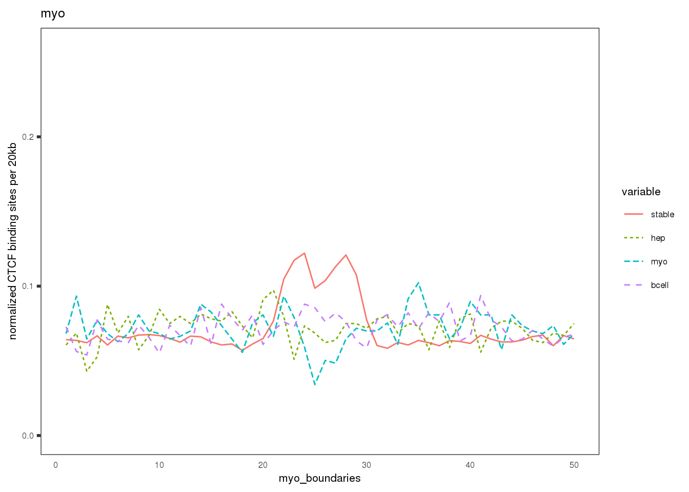
Plot the CBS density distribution around boundaries in three lineages; lineage-conserved and lineage-specific CBS sets.

13.2 Load CBS density data

## Load data
##################################################
file.ls <- list.files('data/countmat/StableSpecificCBS_peakdensity_on_diamondBoundaries/', full.names = T)
file.ls

## [1] "data/countmat/StableSpecificCBS_peakdensity_on_diamondBoundaries//Mouse.stable.specific.CBS.peakDensity_ON_800kbAround_GSE93431_UNTR.50kb.cool.HDF5_diamond-insulation.800kb.1000kb.txt_filter-0.1.matrix"                             
## [2] "data/countmat/StableSpecificCBS_peakdensity_on_diamondBoundaries//Mouse.stable.specific.CBS.peakDensity_ON_800kbAround_GSE98119_Vian-2018-activated_B_cells_24_hours_WT.hic.50kb_diamond-insulation.800kb.1000kb.txt_filter-0.1.matrix"
## [3] "data/countmat/StableSpecificCBS_peakdensity_on_diamondBoundaries//Mouse.stable.specific.CBS.peakDensity_ON_800kbAround_WT_DM.allValidPairs.res50kb_diamond-insulation.800kb.1000kb.txt_filter-0.1.matrix"

13.3 Calculate density

## Section: read the CBS density distribution
##################################################
# absolute density
mat.ls <- lapply(file.ls, function(f){
  df <- fread(f, skip = 1)
  df <- df[, 7:ncol(df)]
  df[is.na(df)] <- 0
  den <- colMeans(df)
  
  n <- ncol(df)
  n.ls <- seq(0,n, length = 5)[-1]
  mat <- data.frame(dist = seq(1,n/4), stable = den[1:n.ls[1]], hep = den[(n.ls[1]+1):n.ls[2]],
                    myo = den[(n.ls[2]+1):n.ls[3]], bcell = den[(n.ls[3]+1):n.ls[4]])
  mat <- melt(mat, id.vars = 'dist')
  
  mat$variable <- factor(mat$variable, levels = c('stable','hep','myo','bcell'))
  mat$value <- as.numeric(as.character(mat$value))
  
 return(mat)
  
  
  
})
# normalized density
mat.ls <- lapply(file.ls, function(f){
  df <- fread(f, skip = 1)
  df <- df[, 7:ncol(df)]
  df[is.na(df)] <- 0
  
  n <- ncol(df)
  n.ls <- seq(0,n, length = 5)[-1]
  
  stable <- df[,1:n.ls[1]]
  hep <- df[, (n.ls[1]+1):n.ls[2]]
  myo <- df[, (n.ls[2]+1):n.ls[3]]
  bcell <- df[, (n.ls[3]+1):n.ls[4]]
  
  stable <- colMeans(stable)/sum(stable)*1e4
  hep <- colMeans(hep)/sum(hep)*1e04
  myo <- colMeans(myo)/sum(myo)*1e04
  bcell <- colMeans(bcell)/sum(bcell)*1e04
  
  mat <- data.frame(dist = seq(1,n/4), stable = stable, hep = hep, myo = myo, bcell = bcell)
  mat <- melt(mat, id.vars = 'dist')
  
  mat$variable <- factor(mat$variable, levels = c('stable','hep','myo','bcell'))
  mat$value <- as.numeric(as.character(mat$value))
  
  return(mat)
  
  
  
})

13.4 Plot

## Section: plot density
##################################################
names(mat.ls) <- c('hep', 'Bcell', 'myo')
mat.ls %>% imap( ~ {
  fontsize = 8
  linesize = 1
  
  df <- .x
  sample <- .y
  
  ggplot(df, aes(x = dist, y = value)) + 
    geom_line(aes(color = variable, linetype = variable))+
    theme_bw() +
    theme(panel.grid.major = element_blank(),panel.grid.minor = element_blank(),
          strip.background = element_blank())+
    theme(text = element_text(size = fontsize), line = element_line(size = linesize),
          axis.ticks.length = unit(.1, "cm"), axis.ticks.x = element_blank()) +
    ylab('normalized CTCF binding sites per 20kb')+ 
    xlab(paste0(sample, '_boundaries'))+ 
    ggtitle(label = sample)+ # labs 
    coord_cartesian(ylim = c(0,0.26))
    
  
})

## $hep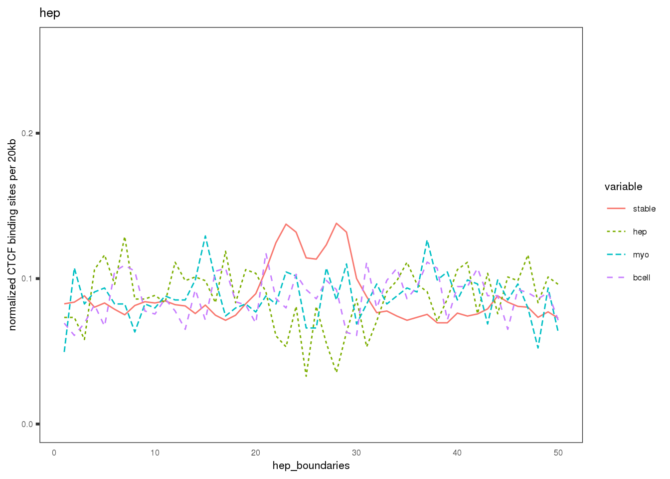

## 
## $Bcell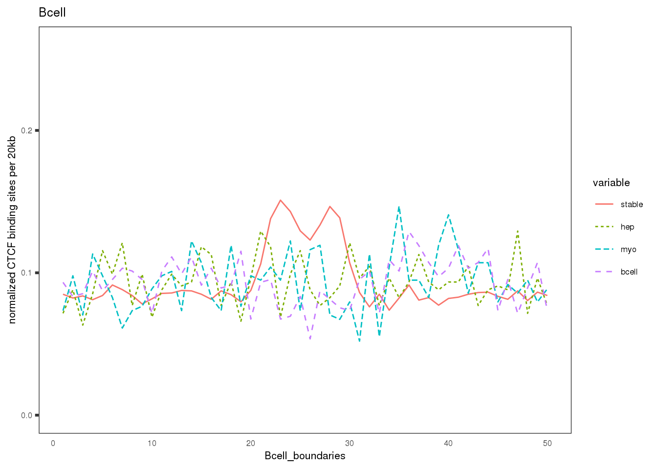

## 
## $myo