Chapter 4 Vehicle mouse
This dataset is high-quality (Virassamy et al. 2023) and includes 7,403 cells from 3 mice treated with vehicle. The cells were labelled using TotalSeqTM anti-mouse hashtag antibodies.
The subset of hash count data is shown below:
## 3 x 10 sparse Matrix of class "dgCMatrix"## [[ suppressing 10 column names 'AAACCTGAGCACCGCT', 'AAACCTGAGGTAGCTG', 'AAACCTGAGTCAATAG' ... ]]##
## mouse1 9957 7 22 23 10 16 12 9 12 10
## mouse2 41 12 12 19 3878 21 21 26 23 11
## mouse3 13 1804 949 2404 7 1739 2106 886 1497 4118The subset of gene expression data is shown below:
## 10 x 10 sparse Matrix of class "dgCMatrix"## [[ suppressing 10 column names 'AAACCTGAGCACCGCT', 'AAACCTGAGGTAGCTG', 'AAACCTGAGTCAATAG' ... ]]##
## Mrpl15 . 2 . 2 2 1 . 2 . .
## Lypla1 . 4 . . 1 1 . . . .
## Gm37988 . . . . . . . . . .
## Tcea1 . 3 . 3 1 . . 1 . 1
## Atp6v1h 2 1 . 1 . 1 . . . .
## Rb1cc1 . 1 . 1 . . 1 . . 2
## 4732440D04Rik . . . . . . . . . .
## Pcmtd1 . . . 1 1 . 2 1 . .
## Gm26901 . . . . . . . . . .
## Rrs1 1 . . 1 . 1 . 1 . .4.1 Local CLR normalization
The first step of CMDdemux is to normalize the hash count data using a local CLR normalization.
##        AAACCTGAGCACCGCT AAACCTGAGGTAGCTG AAACCTGAGTCAATAG AAACCTGAGTGTGGCA AAACCTGCAATGGATA AAACCTGCAGCCTGTG AAACCTGGTACACCGC
## mouse1         4.011845        -1.968127        -1.050141        -1.474977        -1.848995        -1.628752        -1.871388
## mouse2        -1.456617        -1.482620        -1.620686        -1.657298         4.016443        -1.370923        -1.345295
## mouse3        -2.555229         3.450747         2.670827         3.132275        -2.167448         2.999675         3.216683
##        AAACCTGGTTGGGACA AAACCTGGTTTACTCT AAACCTGTCCCATTAT
## mouse1       -1.8261706        -1.786680        -2.004161
## mouse2       -0.8329188        -1.173576        -1.917149
## mouse3        2.6590893         2.960256         3.921310
The output of LocalCLRNorm is a normalized data matrix with rows representing hashtag samples and columns representing cells. Each entry is a normalized value. In addition to downstream demultiplexing, the normalized data can also be used for visualization.
4.2 K-medoids clustering
For high-quality data, we recommend that users use the default parameters directly. The number of clusters equal to the number of hashtags is sufficient for clustering, which is 3 clusters for this dataset.
We then used a boxplot to check whether 3 clusters are appropriate for this data.
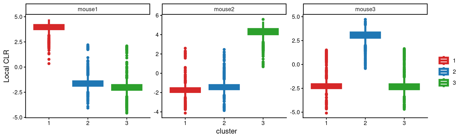
Each hashtag is highly and uniquely expressed in one cluster, which means that three clusters are reasonable for this dataset.
Next, we calculate the Euclidean distance of all cells to their respective cluster centroids.
4.3 Definition of non-core cells
Core cells are defined as cells that are closer to their cluster centroids, while non-core cells are those that are farther away from the cluster centroid. The cut-off between core and non-core cells can be determined using EuclideanDistPlot, which visualizes the cut-off based on the quantile of the distribution via the eu_cut_q parameter, shown as the red line in the plot.
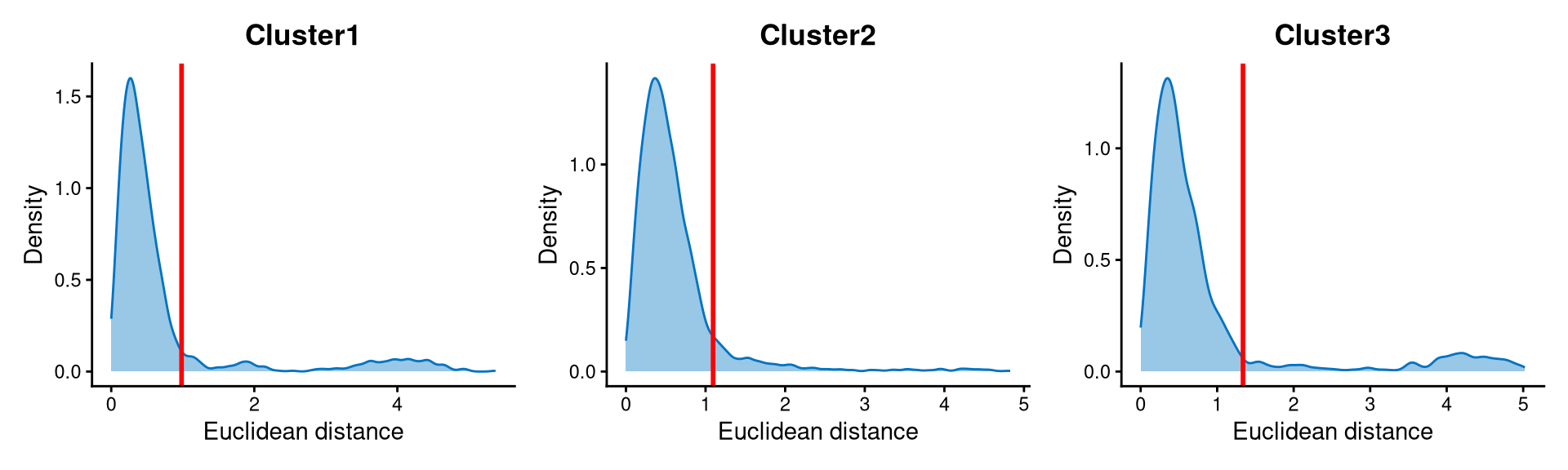
Cells with Euclidean distances larger than the cut-off in the above plot are defined as non-core cells; otherwise, they are core cells. For this dataset, the cut-offs are set at the tails of each distribution.
The cut-offs selected from the plots above are then used to define the non-core cells.
vehicle.noncore <- DefineNonCore(vehicle.cl.dist, vehicle.kmed.cl, eu_cut_q = c(0.86, 0.91, 0.876))
table(vehicle.noncore)
## vehicle.noncore
## Cluster1 Cluster2 Cluster3 non-core
## 1358 3740 1500 805Core cells are labelled by their clusters, and non-core cells are directly labelled as “non-core.”
The definition of core and non-core cells is further examined using CLRPlot.
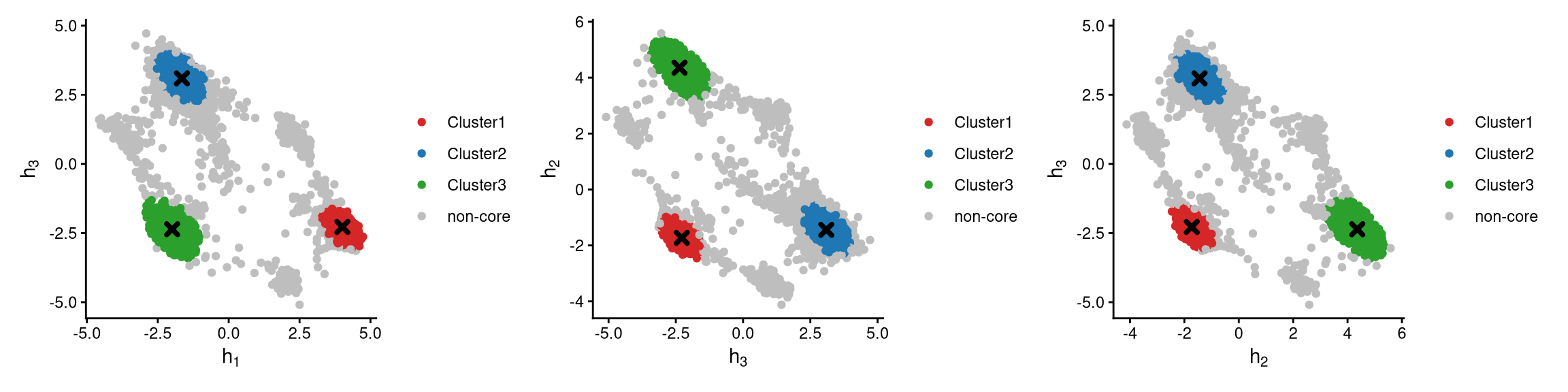
In the plots above, cluster centroids are shown as cross symbols. Core cells cluster around their centroid, while non-core cells lie at the edges of each cluster.
4.4 Label clusters by sample
Each cluster will be labelled with its original sample, and here we use the default medoid-based labelling method.
vehicle.cluster.assign <- LabelClusterHTO(vehicle.clr.norm, vehicle.kmed.cl, vehicle.noncore, label_method = "medoids")
vehicle.cluster.assign
## mouse1 mouse2 mouse3
## 1 3 2The results show each sample and its corresponding cluster index. For example, cluster 1 corresponds to the mouse1 sample.
4.5 Computing the Mahalanobis distance
Using the local CLR-normalized values from LocalCLRNorm, the non-core cell classifications from DefineNonCore, the k-medoids clustering from KmedCluster, and the cluster labelling from LabelClusterHTO, the Mahalanobis distance for each single cell can be calculated using CalculateMD.
vehicle.md.mat <- CalculateMD(vehicle.clr.norm, vehicle.noncore, vehicle.kmed.cl, vehicle.cluster.assign)
vehicle.md.mat[,1:10]
## AAACCTGAGCACCGCT AAACCTGAGGTAGCTG AAACCTGAGTCAATAG AAACCTGAGTGTGGCA AAACCTGCAATGGATA AAACCTGCAGCCTGTG AAACCTGGTACACCGC
## mouse1 1.018919 22.442961 19.123829 20.7899213 24.541071 21.0173792 21.9099836
## mouse2 25.004520 21.675262 21.162644 21.7088676 1.176467 20.8225349 21.0328175
## mouse3 21.547276 1.271012 2.133267 0.8299645 20.035016 0.3086631 0.7830972
## AAACCTGGTTGGGACA AAACCTGGTTTACTCT AAACCTGTCCCATTAT
## mouse1 21.221278 21.3977039 23.169780
## mouse2 19.068649 20.2839111 23.341640
## mouse3 2.115054 0.9427512 2.583675The output is a Mahalanobis distance matrix with rows representing hashtag samples and columns representing cells. Each entry indicates the Mahalanobis distance of a cell to a given hashtag sample.
4.6 Detect outlier cells
Outlier cells, including negatives and doublets, are defined based on the distribution of the minimum Mahalanobis distance across all cells, which can be visualized using MDDensPlot. The cut-off in the plot is determined by the md_cut_q parameter, which specifies the quantile of the distribution and is shown as the red line. Users are encouraged to adjust the cut-off through the md_cut_q parameter.
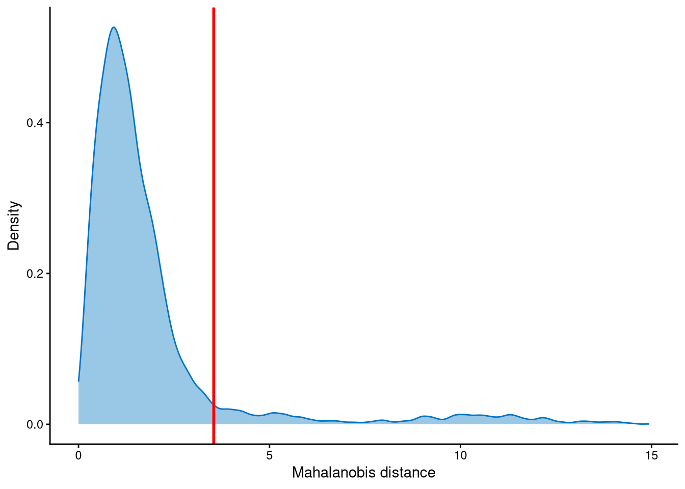
The assumption is that singlets should be closer to the cluster centroids, while outlier cells should be farther away. In this dataset, the distribution is right-skewed with a long tail, so the cut-off is set at the tail to identify outliers.
Outlier cells are then defined using AssignOutlierDrop according to the cut-off selected from the plot.
vehicle.outlier.assign <- AssignOutlierDrop(vehicle.md.mat, md_cut_q = 0.91)
table(vehicle.outlier.assign)
## vehicle.outlier.assign
## Outlier Singlet
## 667 6736In this step, cells are labelled as either outliers or singlets.
4.7 Demultiplexing
The HTO library sizes are used to further distinguish negatives and doublets among the outlier cells. The distribution of HTO library sizes can be visualized using OutlierHTOPlot.
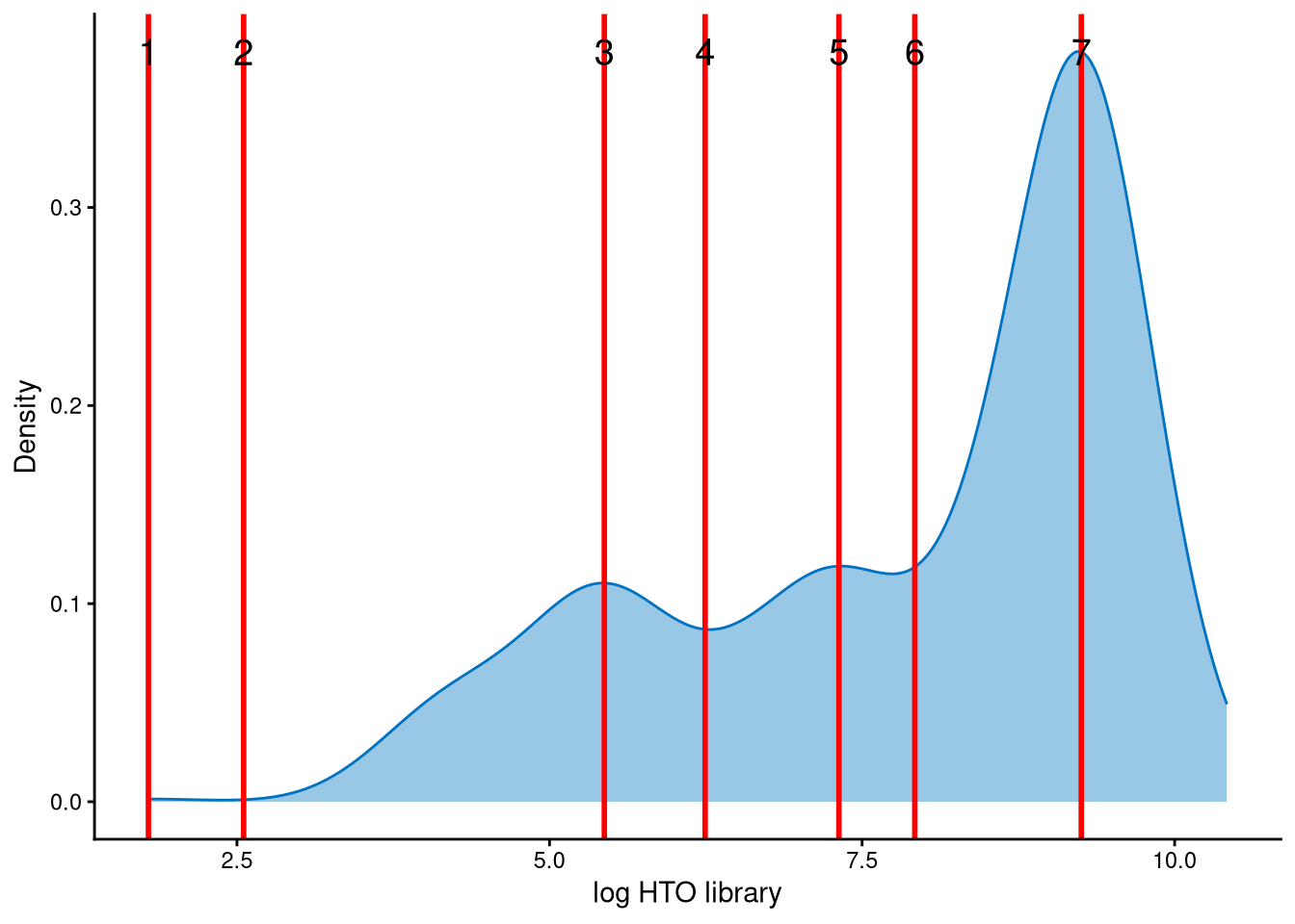
The possible cut-offs for distinguishing negatives and doublets are shown as red vertical lines, representing the modes and anti-modes of the distribution. The distribution is tri-modal, and the default value of the parameter num_modes (the number of modes to detect) is insufficient to capture all modes and anti-modes. Therefore, we set num_modes to 4 for this dataset. Users can then select an appropriate cut-off based on the line index. The assumption is that negative cells have smaller HTO library sizes, whereas doublets have larger HTO library sizes. In this dataset, line index 4 is considered an appropriate cut-off, as it corresponds to an HTO library size of approximately \(e^6=403\). The HTO library size is the total number of hashtag UMIs per cell, and \(e^6\) provides a reasonable threshold for distinguishing negatives from doublets. In contrast, line index 3 corresponds to \(e^{5.2}\approx181\), which is too small, while line index 5 corresponds to \(e^{7.5}\approx1636\), which is too large.
vehicle.cmddemux.assign <- CMDdemuxClass(vehicle.md.mat, vehicle.hash.count, vehicle.outlier.assign, use_gex_data = TRUE, gex.count = vehicle.gex.count, num_modes = 4, cut_no = 4)
head(vehicle.cmddemux.assign)
## demux_id global_class demux_global_class doublet_class
## AAACCTGAGCACCGCT mouse1 Singlet mouse1 mouse1
## AAACCTGAGGTAGCTG mouse3 Singlet mouse3 mouse3
## AAACCTGAGTCAATAG mouse3 Singlet mouse3 mouse3
## AAACCTGAGTGTGGCA mouse3 Singlet mouse3 mouse3
## AAACCTGCAATGGATA mouse2 Singlet mouse2 mouse2
## AAACCTGCAGCCTGTG mouse3 Singlet mouse3 mouse3Gene expression data are available for this dataset, allowing us to use the Mahalanobis distance from CalculateMD, the hashtag count matrix, the outlier classification from AssignOutlierDrop, the gene expression data, and the selected HTO library size cut-off to perform demultiplexing.
CMDdemux provides four types of outputs:
demux_id: the identity for each cell, determined by the sample with the minimum Mahalanobis distance for that cell.
global_class: classification of each cell as Singlet, Doublet, or Negative.
demux_global_class: singlet cells are labeled with their original sample, while negatives and doublets are labeled accordingly.
doublet_class: similar to demux_global_class, but doublets are labeled with their sample of origin. This is particularly useful for combined-hashtag experiments.
##
##  Doublet   mouse1   mouse2   mouse3 Negative
##      364     1441     1545     3905      148
The output above shows the number of cells demultiplexed into each category.