Chapter 6 OT
This dataset is low-quality (Hippen et al. 2023) and includes 9,405 cells from high-grade serous ovarian carcinoma (HGSOC) patients. Batch 2 data is used here, which includes four donors. The cells were labelled using TotalSeqTM-B anti-human hashtag antibodies. The low quality is caused by the excessively strong signals from OT-G.
The subset of hash count data is shown below:
##      AAACCCAAGCAAATCA.1 AAACCCAAGCACTCAT.1 AAACCCAAGGCTTTCA.1 AAACCCACATTCCTAT.1 AAACCCAGTACTCCGG.1 AAACCCAGTAGCGATG.1
## OT-E                 20                  9                  2                 15                  8                 22
## OT-F                614                  4                 75                  5                 13                 12
## OT-G                282                505                 97                219                689                464
## OT-H                 80                 52                 16                249                 92                877
##      AAACCCAGTATCTTCT.1 AAACCCAGTTCAGCTA.1 AAACCCAGTTGCCGAC.1 AAACCCAGTTGGGATG.1
## OT-E                  6                 14                 12                 11
## OT-F                  8                  4                 14                  7
## OT-G                310                670                720                504
## OT-H                380                 83                871               1132
The subset of gene expression data is shown below:
## 10 x 10 sparse Matrix of class "dgCMatrix"## [[ suppressing 10 column names 'AAACCCAAGCAAATCA.1', 'AAACCCAAGCACTCAT.1', 'AAACCCAAGGCTTTCA.1' ... ]]##
## AL627309.1 . . . . . . . . . .
## AL627309.5 . . . . . . . . . .
## AP006222.2 . . . . . . . . . .
## LINC01409 . . . . . . . . 1 .
## FAM87B . . . . . . . . . .
## LINC01128 . . . . . . . 1 1 .
## LINC00115 . . . . . . . . . .
## FAM41C . . . . . . . . . .
## AL645608.6 . . . . . . . . . .
## AL645608.2 . . . . . . . . . .6.1 Local CLR normalization
The first step of CMDdemux is to normalize the hash count data using a local CLR normalization.
##      AAACCCAAGCAAATCA.1 AAACCCAAGCACTCAT.1 AAACCCAAGGCTTTCA.1 AAACCCACATTCCTAT.1 AAACCCAGTACTCCGG.1 AAACCCAGTAGCGATG.1
## OT-E         -1.8319878          -1.224628         -2.1132693          -1.097270         -1.7791687          -1.519538
## OT-F          1.5451121          -1.917775          1.1188517          -2.078100         -1.3373359          -2.090083
## OT-G          0.7689367           2.699324          1.3730859           1.523768          2.5602983           1.487006
## OT-H         -0.4820610           0.443079         -0.3786683           1.651602          0.5562062           2.122615
##      AAACCCAGTATCTTCT.1 AAACCCAGTTCAGCTA.1 AAACCCAGTTGCCGAC.1 AAACCCAGTTGGGATG.1
## OT-E          -2.010522         -1.1062183          -2.091158          -1.970476
## OT-F          -1.759207         -2.2048306          -1.948057          -2.375941
## OT-G           1.783361          2.6945006           1.924532           1.769176
## OT-H           1.986368          0.6165483           2.114682           2.577242
The output of LocalCLRNorm is a normalized data matrix with rows representing hashtag samples and columns representing cells. Each entry is a normalized value.
6.2 K-medoids clustering
The local CLR-normalized values are used here for K-medoids clustering. Since this dataset has four samples, the default parameters are applied, which divides the cells into four clusters.
A boxplot is then used to check whether four clusters are appropriate for this dataset.
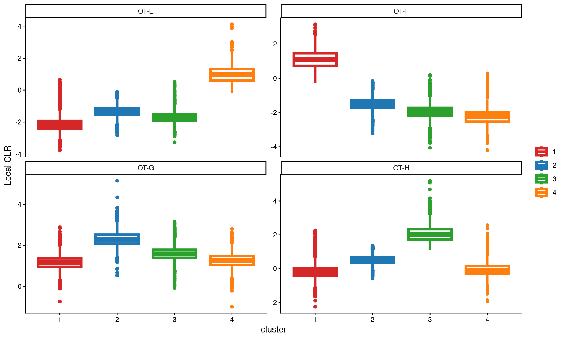
The box plot shows that each hashtag sample is highly and uniquely expressed in one cluster, indicating that four clusters are ideal for this dataset.
Next, the Euclidean distance between cells and their corresponding cluster centroid within each cluster is calculated using EuclideanClusterDist.
6.3 Definition of non-core cells
Core cells are defined as cells that are closer to their cluster centroids, while non-core cells are those that are farther away from the cluster centroid. The cut-off between core and non-core cells can be determined using EuclideanDistPlot, which visualizes the cut-off based on the quantile of the distribution via the eu_cut_q parameter, shown as the red line in the plot.
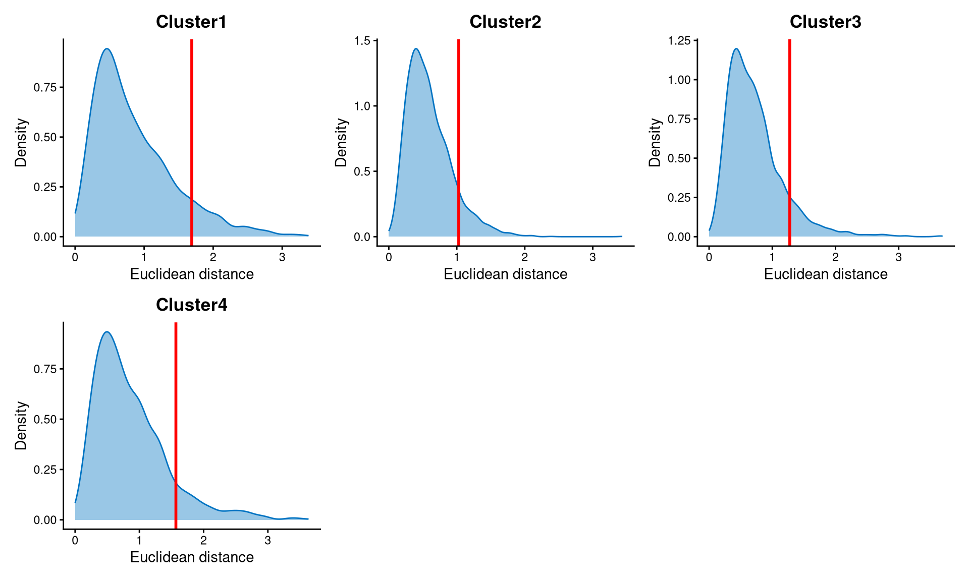
We use the default value to set the cut-offs for non-core cells, which is the 0.9 quantile of the distribution. From the plot, the cut-off for each cluster is located at the tail of the distribution. Cells with Euclidean distances larger than the cut-off are defined as non-core cells, and the others are core cells.
Core and non-core cells are then classified using DefineNonCore, applying the default parameter selected from the above plot.
## otb2.noncore
## Cluster1 Cluster2 Cluster3 Cluster4 non-core
##     1530     3603     2052     1279      941
Core cells are labelled by their clusters, and non-core cells are directly labelled as “non-core.”
The definition of core and non-core cells is further examined using CLRPlot.
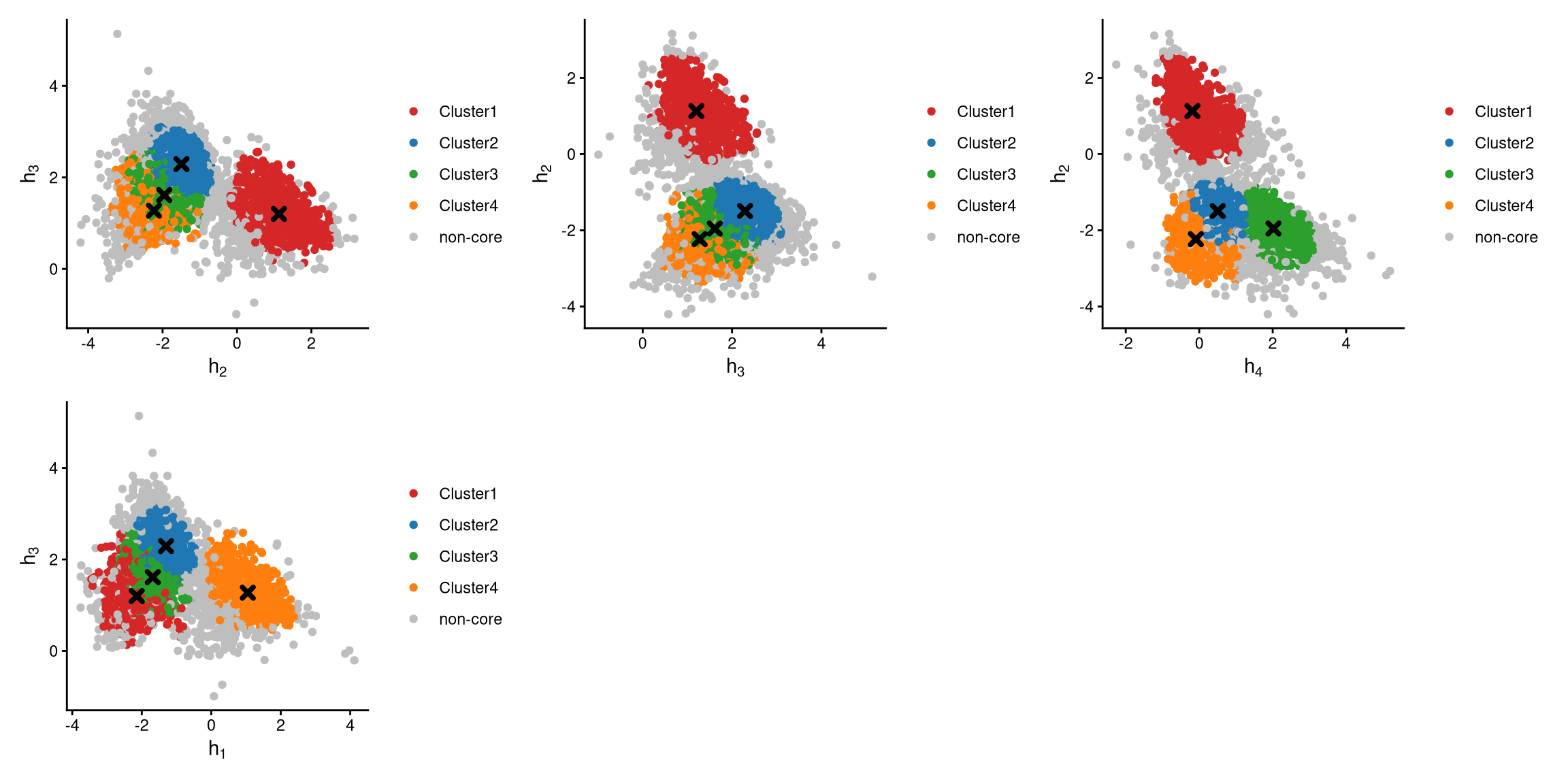
The pairwise local CLR-normalized values are shown in the plots above. The cluster centroids are indicated by cross signs. It is clear that core cells cluster around the centroids, whereas non-core cells lie at the edges of the clusters.
6.4 Label clusters by sample
Each cluster will be labelled with its original sample, and here we use the default medoid-based labelling method.
otb2.cluster.assign <- LabelClusterHTO(otb2.clr.norm, otb2.kmed.cl, otb2.noncore, label_method = "medoids")
otb2.cluster.assign
## OT-E OT-F OT-G OT-H
## 4 1 2 3The results show each sample and its corresponding cluster index. For example, cluster 1 corresponds to the OT-F sample.
6.5 Computing the Mahalanobis distance
Using the local CLR-normalized values from LocalCLRNorm, the non-core cell classifications from DefineNonCore, the k-medoids clustering from KmedCluster, and the cluster labelling from LabelClusterHTO, the Mahalanobis distance for each single cell can be calculated using CalculateMD.
otb2.md.mat <- CalculateMD(otb2.clr.norm, otb2.noncore, otb2.kmed.cl, otb2.cluster.assign)
otb2.md.mat[,1:10]
## AAACCCAAGCAAATCA.1 AAACCCAAGCACTCAT.1 AAACCCAAGGCTTTCA.1 AAACCCACATTCCTAT.1 AAACCCAGTACTCCGG.1 AAACCCAGTAGCGATG.1
## OT-E 11.392181 7.217335 11.0612110 7.011771 8.450403 8.5696230
## OT-F 1.907845 8.638579 0.6983818 9.087203 7.156417 9.5230127
## OT-G 8.665586 1.541855 7.1774731 3.904002 1.479951 4.9047101
## OT-H 10.460539 5.179151 9.3390877 1.784838 4.799226 0.6788606
## AAACCCAGTATCTTCT.1 AAACCCAGTTCAGCTA.1 AAACCCAGTTGCCGAC.1 AAACCCAGTTGGGATG.1
## OT-E 9.493626 7.036342 9.870229 10.256178
## OT-F 8.724617 9.330447 9.329814 10.724126
## OT-G 4.423268 2.073863 4.747158 6.026136
## OT-H 1.062285 4.955189 1.385506 1.899232The output is a Mahalanobis distance matrix with rows representing hashtag samples and columns representing cells. Each entry indicates the Mahalanobis distance of a cell to a given hashtag sample.
6.6 Detect outlier cells
Outlier cells, including negatives and doublets, are defined based on the distribution of the minimum Mahalanobis distance across all cells, which can be visualized using MDDensPlot. The cut-off in this dataset is determined using the md_auto parameter. When md_auto is set to TRUE, the cut-off is defined as the 0.975 quantile of a chi-square distribution, because the Mahalanobis distance is assumed to follow a chi-square distribution.
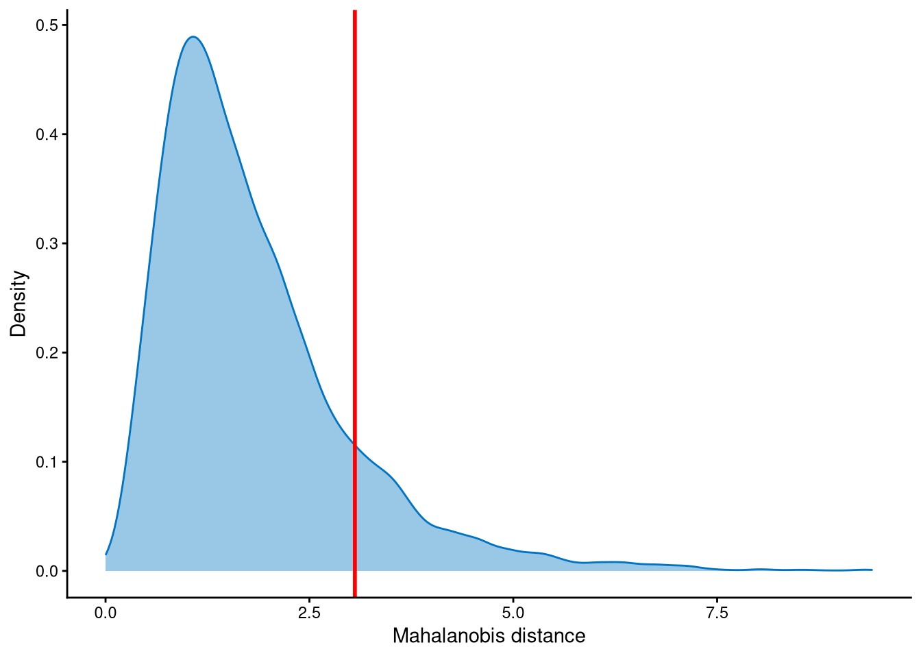
The distribution of Mahalanobis distance is right-skewed. The cut-off to select outlier cells is defined by the default parameter of md_auto. The cut-off is set at the tail of the distribution. Cells with Mahalanobis distance larger than the cut-off will be defined as outliers, and others are defined as singlets.
Outlier cells are then defined using AssignOutlierDrop according to the cut-off selected from the plot.
## otb2.outlier.assign
## Outlier Singlet
##    1202    8203
In this step, cells are labelled as either outliers or singlets.
6.7 Demultiplexing
The HTO library sizes are used to further distinguish negatives and doublets among the outlier cells. The distribution of HTO library sizes can be visualized using OutlierHTOPlot. The possible cut-offs corresponding to the modes and anti-modes are shown as red lines in the plot.
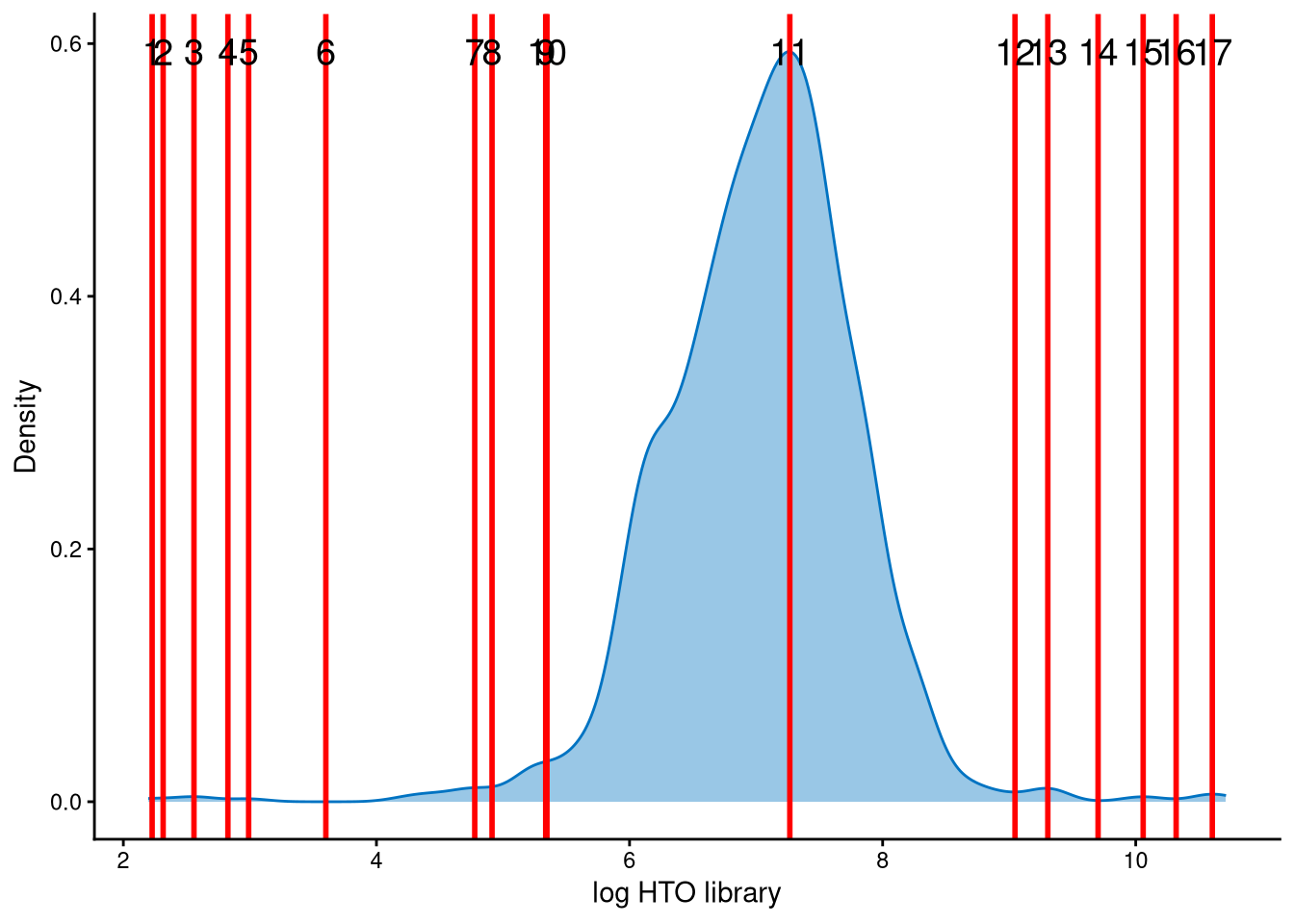
The distribution of HTO library sizes is not classically bimodal. Different values of the parameter num_modes have been tested on the data, and line index 10 is an appropriate cut-off to distinguish negatives and doublets. The HTO library size (total hashtag counts per cell) at line index 10 is approximately \(e^{5.8}\approx330\), which is a reasonable cut-off.
In the final step of demultiplexing, the Mahalanobis distance from CalculateMD, the original hashtag count matrix, the outlier classifications from AssignOutlierDrop, the gene expression data, and the selected HTO library size cut-off from the above plot are applied.
otb2.cmddemux.assign <- CMDdemuxClass(otb2.md.mat, otb2.hash.count, otb2.outlier.assign, use_gex_data = TRUE, gex.count = otb2.gex.count, num_modes = 9, cut_no = 10)
head(otb2.cmddemux.assign)
## demux_id global_class demux_global_class doublet_class
## AAACCCAAGCAAATCA.1 OT-F Singlet OT-F OT-F
## AAACCCAAGCACTCAT.1 OT-G Singlet OT-G OT-G
## AAACCCAAGGCTTTCA.1 OT-F Singlet OT-F OT-F
## AAACCCACATTCCTAT.1 OT-H Singlet OT-H OT-H
## AAACCCAGTACTCCGG.1 OT-G Singlet OT-G OT-G
## AAACCCAGTAGCGATG.1 OT-H Singlet OT-H OT-HCMDdemux provides four types of outputs:
demux_id: the identity for each cell, determined by the sample with the minimum Mahalanobis distance for that cell.
global_class: classification of each cell as Singlet, Doublet, or Negative.
demux_global_class: singlet cells are labeled with their original sample, while negatives and doublets are labeled accordingly.
doublet_class: similar to demux_global_class, but doublets are labeled with their sample of origin. This is particularly useful for combined-hashtag experiments.
##
##  Doublet Negative     OT-E     OT-F     OT-G     OT-H
##      799       17     1211     1445     3861     2072
The output above shows the number of cells demultiplexed into each category.