Chapter 3 BAL
This dataset is high-quality (Howitt et al. 2023) and includes 24,804 cells from 8 pediatric bronchoalveolar lavage (BAL) fluid donors. Cells were labelled using TotalSeq-A antibodies. Only Batch 1 data is shown here. The gene expression data are not available.
The subset of hash count data is shown below:
##       X1_AAACCCACACTTCCTG.1 X1_AAACCCACAGACAAAT.1 X1_AAACCCACAGGACGAT.1 X1_AAACCCACATCCTAAG.1 X1_AAACCCAGTAACATCC.1
## BAL-A                    18                    15                     9                     8                    18
## BAL-B                    15                    12                    17                    28                    26
## BAL-C                    12                   202                    11                    20                    14
## BAL-D                   284                     1                   239                   219                     9
## BAL-E                    11                     5                     7                    12                   746
## BAL-F                     4                     6                     3                    13                    11
## BAL-G                     8                     8                     4                     7                    11
## BAL-H                    17                    10                    15                    21                    27
##       X1_AAACCCAGTACAGTTC.1 X1_AAACCCAGTACTGTTG.1 X1_AAACCCAGTGTCACAT.1 X1_AAACCCAGTTCTCAGA.1 X1_AAACCCAGTTGTCATG.1
## BAL-A                    28                    15                    22                     7                   296
## BAL-B                    20                  1424                    26                   336                    27
## BAL-C                    11                     7                    11                     8                    11
## BAL-D                     7                     3                    19                     2                     1
## BAL-E                    10                    13                    48                     3                     7
## BAL-F                     5                     8                    10                     1                     2
## BAL-G                   768                     6                     9                     2                    10
## BAL-H                    20                    19                   776                     9                    14
3.1 Local CLR normalization
The first step of CMDdemux is to normalize the hash count data using a local CLR normalization.
##       X1_AAACCCACACTTCCTG.1 X1_AAACCCACAGACAAAT.1 X1_AAACCCACAGGACGAT.1 X1_AAACCCACATCCTAAG.1 X1_AAACCCAGTAACATCC.1
## BAL-A          0.0548880871            0.31300363            -0.3231980          -0.849920557           -0.32668529
## BAL-B         -0.1169621698            0.10536427             0.2645886           0.320150696            0.02471260
## BAL-C         -0.3246015346            2.85362089            -0.1408765          -0.002622696           -0.56307407
## BAL-D          2.7629382882           -1.76643791             2.8548558           2.346482412           -0.96853917
## BAL-E         -0.4046442423           -0.66782562            -0.5463416          -0.482195777            3.34494092
## BAL-F         -1.2801129796           -0.51367494            -1.2394888          -0.408087805           -0.78621762
## BAL-G         -0.6923263147           -0.26236051            -1.0163452          -0.967703593           -0.78621762
## BAL-H          0.0008208658           -0.06168982             0.1468056           0.043897319            0.06108024
##       X1_AAACCCAGTACAGTTC.1 X1_AAACCCAGTACTGTTG.1 X1_AAACCCAGTGTCACAT.1 X1_AAACCCAGTTCTCAGA.1 X1_AAACCCAGTTGTCATG.1
## BAL-A            0.26036650           -0.13718328           -0.25946966          -0.005058491            3.13273342
## BAL-B           -0.06240689            4.35215509           -0.09912701           3.735582898            0.77120579
## BAL-C           -0.62202268           -0.83033046           -0.91005723           0.112724545           -0.07609207
## BAL-D           -1.02748778           -1.52347764           -0.39923160          -0.985887744           -1.86785154
## BAL-E           -0.70903405           -0.27071468            0.49685642          -0.698205672           -0.48155718
## BAL-F           -1.31516986           -0.71254743           -0.99706860          -1.391352852           -1.46238643
## BAL-G            3.53816164           -0.96386186           -1.09237878          -0.985887744           -0.16310345
## BAL-H           -0.06240689            0.08596027            3.26047647           0.218085060            0.14705148
The output of LocalCLRNorm is a normalized data matrix with rows representing hashtag samples and columns representing cells. Each entry is a normalized value.
3.2 K-medoids clustering
For high-quality data, we recommend that users use the default parameters directly. The number of clusters equal to the number of hashtags is sufficient for clustering, which is 8 clusters for this dataset.
We then used a boxplot to check whether 8 clusters are appropriate for this data.
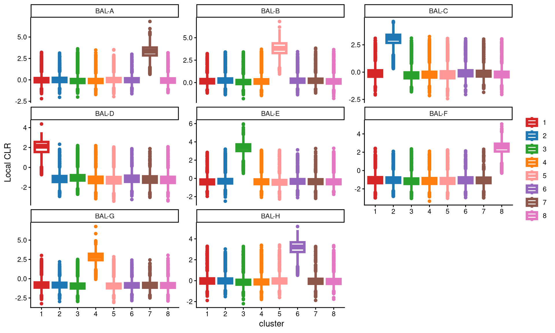
It is quite apparent that each hashtag is uniquely and highly expressed in a single cluster. Therefore, 8 clusters are sufficient for this dataset.
Next, we calculate the Euclidean distance of all cells to their respective cluster centroids.
3.3 Definition of non-core cells
The distribution of these distances is then examined using EuclideanDistPlot. The cut-off for each cluster is determined by the eu_cut_q parameter, which represents the quantile of the distribution. We recommend that users select a value in the tail of the distribution and adjust the parameter by visualizing the red line in each plot.
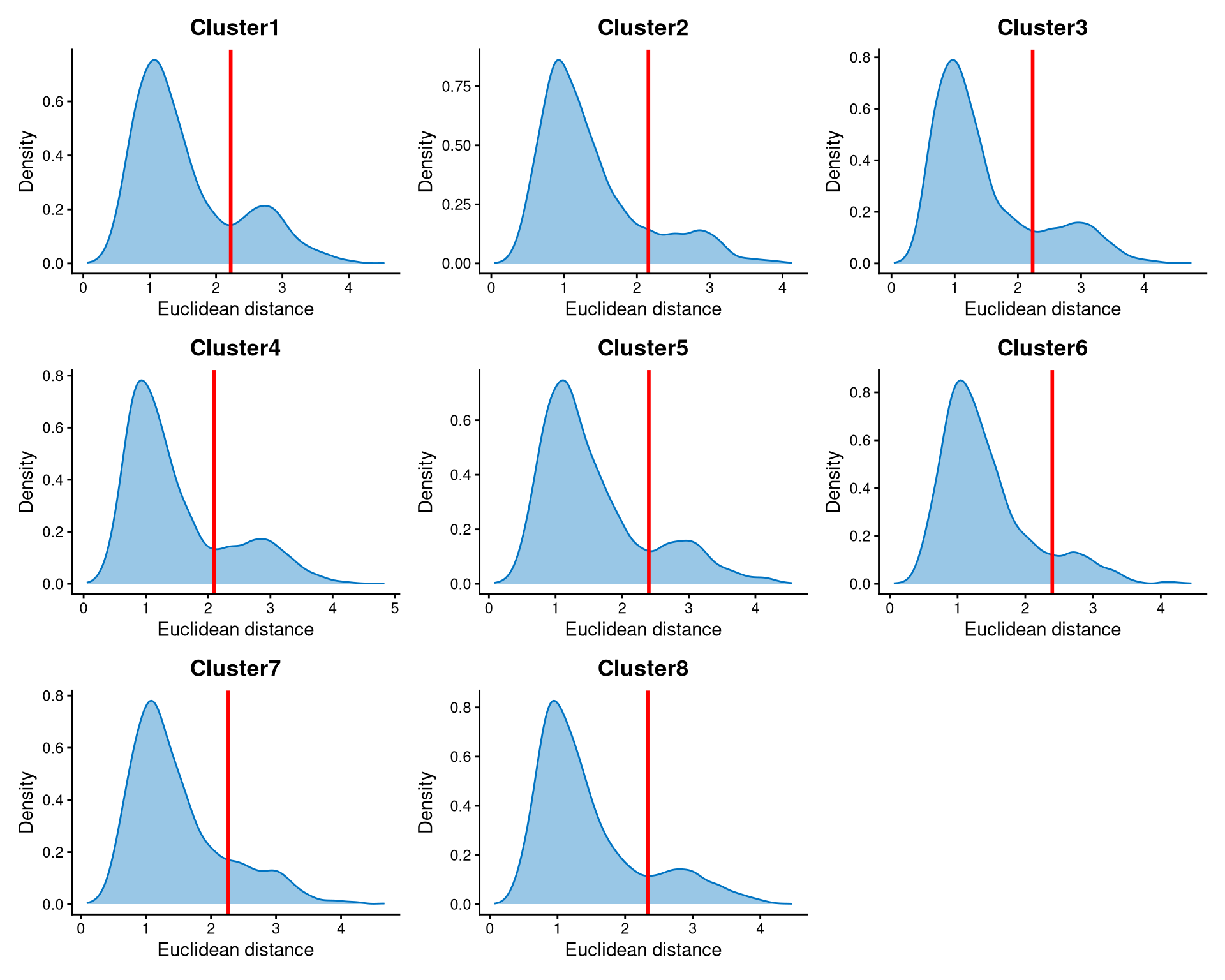
The Euclidean distances within each cluster are bimodally distributed. The peak with smaller distances corresponds to core cells, which are closer to the cluster centroid, while the peak with larger distances corresponds to non-core cells, which are further away. The cut-off for each cluster is chosen at the anti-mode of the distribution.
The non-core cells are defined by the DefineNonCore function, using the Euclidean distance output from EuclideanClusterDist, the k-medoids clustering output from KmedCluster, and the cut-offs examined from EuclideanDistPlot.
balb1.noncore <- DefineNonCore(balb1.cl.dist, balb1.kmed.cl, eu_cut_q = c(0.79, 0.85, 0.81, 0.78, 0.83, 0.89, 0.84, 0.84))
table(balb1.noncore)
## balb1.noncore
## Cluster1 Cluster2 Cluster3 Cluster4 Cluster5 Cluster6 Cluster7 Cluster8 non-core
## 2202 3436 3044 2490 2912 2575 1712 2166 4267Core cells are labelled according to their cluster, while non-core cells are labelled as “non-core.”
The classified core and non-core cells are then examined using CLRPlot.
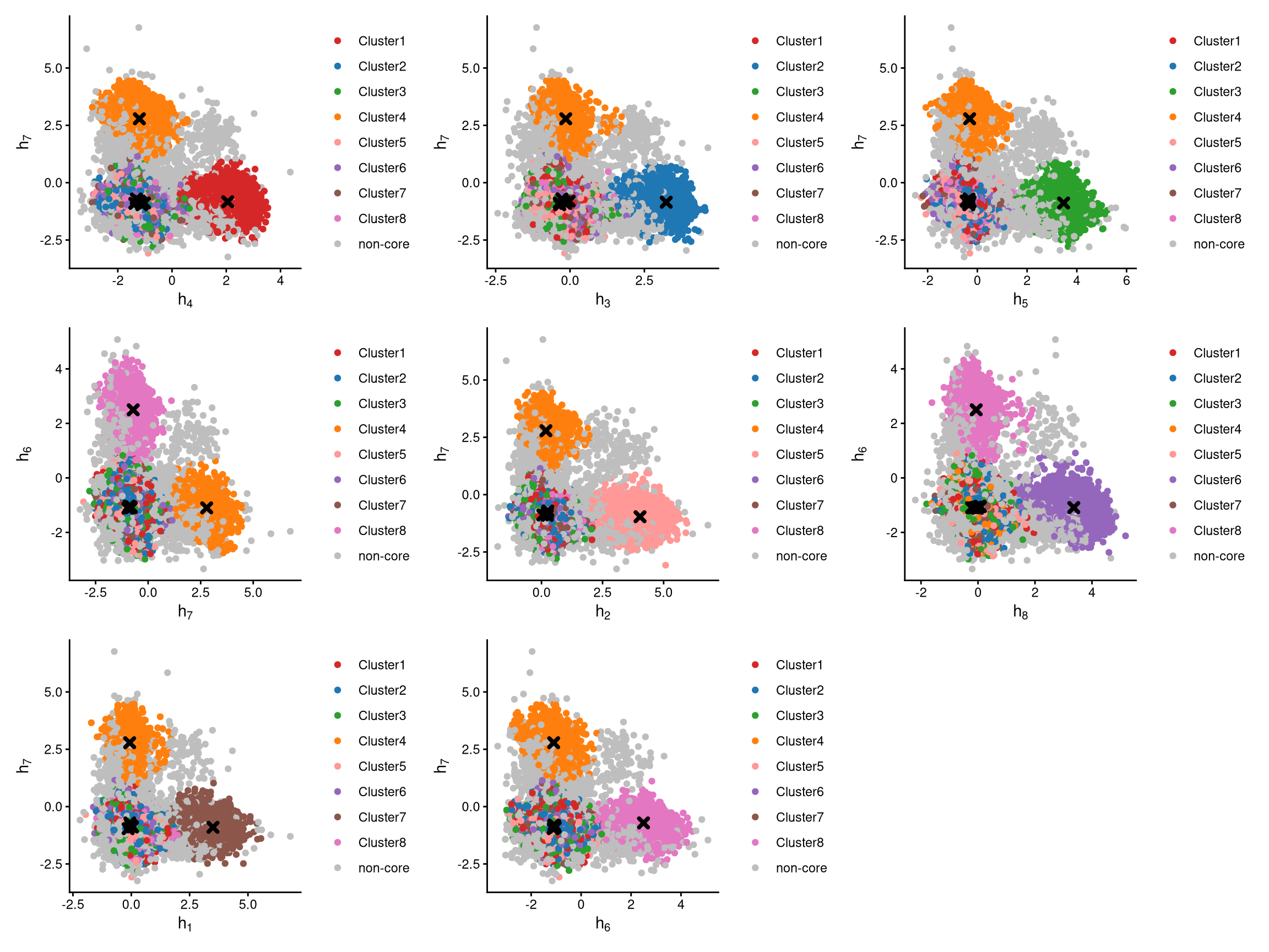
The plots above show pairwise CLR-normalized values within each cell. The cluster centroids are indicated by black cross symbols. In these plots, non-core cells are located farther from their cluster centroids, while core cells are closer, as expected.
3.4 Label clusters by sample
For each cluster, its sample of origin can be assigned using LabelClusterHTO with CLR-normalized values from LocalCLRNorm, k-medoids clustering from KmedCluster, and non-core cells from DefineNonCore. Generally, the default value of the label_method parameter works for most datasets. If it does not, the alternative value “expression” is recommended.
balb1.cluster.assign <- LabelClusterHTO(balb1.clr.norm, balb1.kmed.cl, balb1.noncore, label_method = "medoids")
balb1.cluster.assign
## BAL-A BAL-B BAL-C BAL-D BAL-E BAL-F BAL-G BAL-H
## 7 5 2 1 3 8 4 6The output shows each hashtag sample and its corresponding cluster index.
3.5 Computing the Mahalanobis distance
The Mahalanobis distance for each single cell can be calculated via CalculateMD.
balb1.md.mat <- CalculateMD(balb1.clr.norm, balb1.noncore, balb1.kmed.cl, balb1.cluster.assign)
balb1.md.mat[,1:10]
## X1_AAACCCACACTTCCTG.1 X1_AAACCCACAGACAAAT.1 X1_AAACCCACAGGACGAT.1 X1_AAACCCACATCCTAAG.1 X1_AAACCCAGTAACATCC.1
## BAL-A 10.927815 10.237574 11.667071 12.028096 12.168967
## BAL-B 11.479211 11.179391 10.945886 10.323254 12.297034
## BAL-C 11.159726 2.413062 10.980606 10.231049 12.005398
## BAL-D 1.707717 10.272518 1.882647 2.478202 10.470651
## BAL-E 11.687767 12.055713 12.129021 11.577098 1.381756
## BAL-F 10.986433 9.444398 11.074167 9.340607 10.610735
## BAL-G 10.288890 9.141810 10.859263 10.242215 10.917122
## BAL-H 10.780809 10.398264 10.657356 10.287044 11.569898
## X1_AAACCCAGTACAGTTC.1 X1_AAACCCAGTACTGTTG.1 X1_AAACCCAGTGTCACAT.1 X1_AAACCCAGTTCTCAGA.1 X1_AAACCCAGTTGTCATG.1
## BAL-A 11.466232 12.320324 11.732997 11.209385 2.405890
## BAL-B 12.601233 1.717611 12.149781 1.681982 10.589038
## BAL-C 12.236479 12.525331 12.392677 10.207126 10.570715
## BAL-D 10.489353 11.107960 9.083088 9.470056 10.250325
## BAL-E 12.819532 12.833288 10.682070 12.691715 11.697810
## BAL-F 11.282977 10.774135 10.714846 10.820999 10.845493
## BAL-G 2.321026 11.743999 11.326663 10.822682 9.465207
## BAL-H 11.674930 11.861854 3.475674 10.625543 10.571685The output is a Mahalanobis distance matrix. Each row of the matrix represents a hashtag sample, and each column represents a cell. Each entry of the matrix represents the Mahalanobis distance of the cell to the sample.
3.6 Detect outlier cells
Outlier cells are negatives and doublets. They are identified based on the distribution of the minimum Mahalanobis distance across all cells, which can be visualized using MDDensPlot. The cut-off is determined by the md_cut_q parameter, representing the quantile of the distribution. The red line in the plot indicates the cut-off. We recommend that users adjust the md_cut_q parameter to find an optimal cut-off between singlets and outliers.
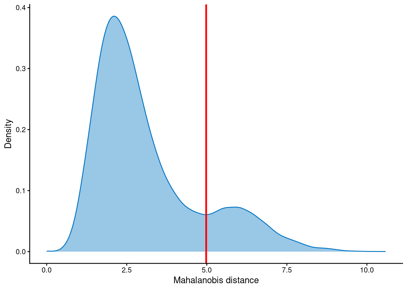
The Mahalanobis distances are clearly bimodally distributed. The peak with smaller Mahalanobis distances corresponds to singlets, while the peak with larger distances corresponds to outlier cells. The cut-off should be set at the anti-mode of this distribution.
The selected cut-off can then be used to define outlier cells via AssignOutlierDrop.
balb1.outlier.assign <- AssignOutlierDrop(balb1.md.mat, md_cut_q = 0.84)
table(balb1.outlier.assign)
## balb1.outlier.assign
## Outlier Singlet
## 3969 20835The output of AssignOutlierDrop assigns each cell as either “Outlier” or “Singlet”.”
3.7 Demultiplexing
The HTO library sizes are used to further distinguish negatives and doublets within the outlier cells. The distribution of HTO library sizes can be visualized using OutlierHTOPlot. The library sizes are generally multimodally distributed, and the num_modes parameter specifies the number of modes in the distribution.
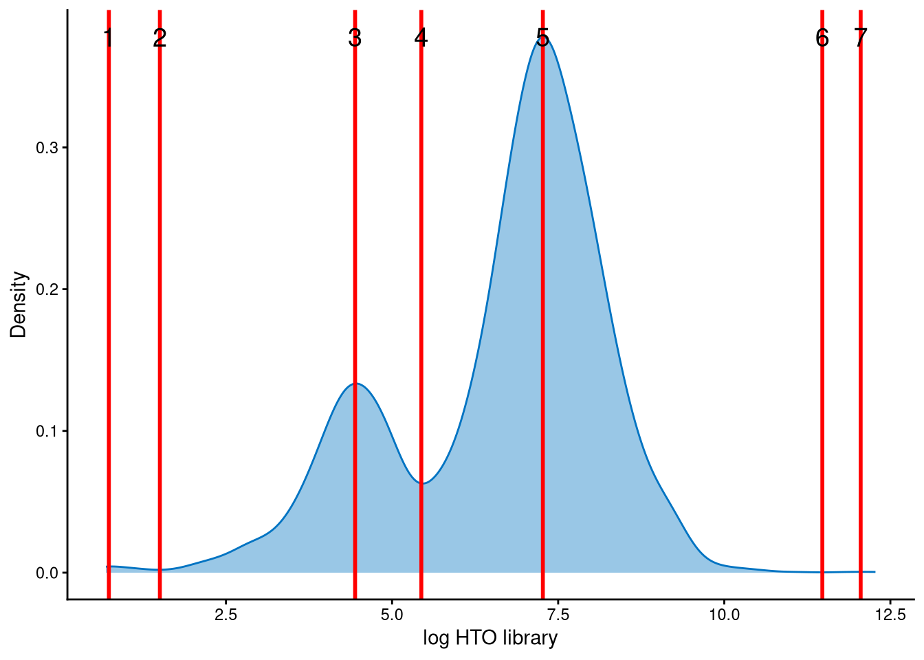
In this dataset, the HTO library sizes for outlier cells are bimodally distributed. The mode with smaller library sizes corresponds to potential negatives, while the mode with larger library sizes corresponds to potential doublets. The red lines represent the modes and anti-modes of the distribution. The red line with index 4 is an appropriate cut-off for distinguishing negatives and doublets among the outlier cells.
balb1.cmddemux.assign <- CMDdemuxClass(balb1.md.mat, balb1.hash.count, balb1.outlier.assign, num_modes = 4, cut_no = 4)
head(balb1.cmddemux.assign)
## demux_id global_class demux_global_class doublet_class
## X1_AAACCCACACTTCCTG.1 BAL-D Singlet BAL-D BAL-D
## X1_AAACCCACAGACAAAT.1 BAL-C Singlet BAL-C BAL-C
## X1_AAACCCACAGGACGAT.1 BAL-D Singlet BAL-D BAL-D
## X1_AAACCCACATCCTAAG.1 BAL-D Singlet BAL-D BAL-D
## X1_AAACCCAGTAACATCC.1 BAL-E Singlet BAL-E BAL-E
## X1_AAACCCAGTACAGTTC.1 BAL-G Singlet BAL-G BAL-GSince gene expression data is not available for this dataset, only cell hashing data is used for demultiplexing. The num_modes parameter can be determined using OutlierHTOPlot, and the cut_no parameter is selected based on the index of the appropriate red line in the plot.
CMDdemux provides four types of outputs:
demux_id: the identity for each cell, determined by the sample with the minimum Mahalanobis distance for that cell.
global_class: classification of each cell as Singlet, Doublet, or Negative.
demux_global_class: singlet cells are labeled with their original sample, while negatives and doublets are labeled accordingly.
doublet_class: similar to demux_global_class, but doublets are labeled with their sample of origin. This is particularly useful for combined-hashtag experiments.
##
##    BAL-A    BAL-B    BAL-C    BAL-D    BAL-E    BAL-F    BAL-G    BAL-H  Doublet Negative
##     1737     2883     3520     2282     3076     2176     2611     2550     3071      898
The output above shows the number of cells demultiplexed into each category.