Chapter 7 EMBRYO MULTI-Seq LMO
This dataset is low quality (Brown et al. 2024) and includes 9,745 cells from embryonic day 18.5 mouse brain. All cells originate from a single mouse and were partitioned into 12 replicates labelled using MULTI-Seq lipid-modified oligos (LMO). The low quality is due to MULTI_2 failing to label cells, which is considered an unlabelled hash because it labels only a small number of cells.
The subset of hash count data is shown below:
## 12 x 10 sparse Matrix of class "dgCMatrix"## [[ suppressing 10 column names 'AAACCCAAGAACTGAT-1', 'AAACCCAAGATGAAGG-1', 'AAACCCAAGGGTCTTT-1' ... ]]##
## MULTI_2 . . . 1 . . . 3 10 .
## MULTI_3 3 1 3 1 7 8 . 6 4 .
## MULTI_4 28 24 82 33 50 19 30 77 37 15
## MULTI_5 15 20 47 29 32 23 24 22 31 17
## MULTI_6 23 19 76 33 46 391 29 76 57 47
## MULTI_7 6 9 7 336 7 3 1 126 2 .
## MULTI_8 38 37 1544 125 75 71 58 3374 63 57
## MULTI_9 3 4 20 10 10 34 3 6 11 2
## MULTI_10 67 8 43 16 31 1340 17 18 18 5
## MULTI_11 10 117 17 29 15 3971 10 49 28 10
## MULTI_12 14 10 17 13 7 26 19 15 215 3
## MULTI_13 13 15 265 23 25 8 27 73 28 21The subset of gene expression data is shown below:
## 10 x 10 sparse Matrix of class "dgCMatrix"## [[ suppressing 10 column names 'AAACCCAAGAACTGAT-1', 'AAACCCAAGATGAAGG-1', 'AAACCCAAGGGTCTTT-1' ... ]]##
## Xkr4 . 1 . . . . . . 1 .
## Gm1992 . . . . . . . . . .
## Gm19938 1 2 . . 1 1 . . 2 .
## Gm37381 . . . . . . . . . .
## Rp1 . . . . . . . . . .
## Sox17 . . . . . . . . . .
## Gm37587 . . . . . . . . . .
## Gm37323 . . . . . . . . . .
## Mrpl15 1 . . . . 1 . . . .
## Lypla1 . . . 1 . . . . . .7.1 Local CLR normalization
The first step of CMDdemux is to normalize the hash count data using a local CLR normalization.
##          AAACCCAAGAACTGAT-1 AAACCCAAGATGAAGG-1 AAACCCAAGGGTCTTT-1 AAACCCAAGTTGAAGT-1 AAACCCACAGAGTTCT-1 AAACCCACATAATGAG-1
## MULTI_2         -2.47204245        -2.47002334         -3.4696095        -2.38568572        -2.81182127         -3.7118199
## MULTI_3         -1.08574809        -1.77687616         -2.0833151        -2.38568572        -0.73237972         -1.5145953
## MULTI_4          0.89525338         0.74885248          0.9492311         0.44752763         1.12000437         -0.7160876
## MULTI_5          0.30054627         0.57449910          0.4015915         0.32236448         0.68468630         -0.5337660
## MULTI_6          0.70601138         0.52570893          0.8741959         0.44752763         1.03832634          2.2594420
## MULTI_7         -0.52613230        -0.16743825         -1.3901680         2.74125003        -0.73237972         -2.3255255
## MULTI_8          1.19151920         1.16756282          3.8731697         1.75744901         1.51891207          0.5648463
## MULTI_9         -1.08574809        -0.86058543         -0.4250871        -0.68093763        -0.41392599         -0.1564718
## MULTI_10         1.74746525        -0.27279876          0.3145801        -0.24561955         0.65391464          3.4893510
## MULTI_11        -0.07414718         2.30066128         -0.5792377         0.32236448        -0.03923254          4.5752052
## MULTI_12         0.23600775        -0.07212807         -0.5792377        -0.43977557        -0.73237972         -0.4159830
## MULTI_13         0.16701488         0.30256538          2.1138868         0.09922093         0.44627527         -1.5145953
##          AAACCCAGTACTAGCT-1 AAACCCAGTCGTAATC-1 AAACCCAGTGTGATGG-1 AAACCCATCAGATGCT-1
## MULTI_2         -2.31893693         -2.2816704         -0.7660888         -1.9466840
## MULTI_3         -2.31893693         -1.7220546         -1.5545462         -1.9466840
## MULTI_4          1.11505027          0.6887441          0.4736020          0.8259047
## MULTI_5          0.89993889         -0.5324705          0.3017518          0.9436877
## MULTI_6          1.08226045          0.6758407          0.8964589          1.9245170
## MULTI_7         -1.62578975          1.1762224         -2.0653718         -1.9466840
## MULTI_8          1.75860051          4.4561859          0.9948990          2.1137590
## MULTI_9         -0.93264257         -1.7220546         -0.6790775         -0.8480717
## MULTI_10         0.57143482         -0.7235257         -0.2195451         -0.1549246
## MULTI_11         0.07895834          0.2440583          0.2033117          0.4512112
## MULTI_12         0.67679534         -0.8953760          2.2112943         -0.5603897
## MULTI_13         1.01326758          0.6361004          0.2033117          1.1443584
The output of LocalCLRNorm is a normalized data matrix with rows representing hashtag samples and columns representing cells. Each entry is a normalized value.
7.2 K-medoids clustering
The local CLR-normalized values are used here for K-medoids clustering. Since this dataset has twelve samples, the default parameters are initially applied, which divide the cells into twelve clusters.
We use a boxplot to check whether the number of clusters is appropriate for clustering. An ideal result is that one box should be significantly higher than the other boxes in each panel.
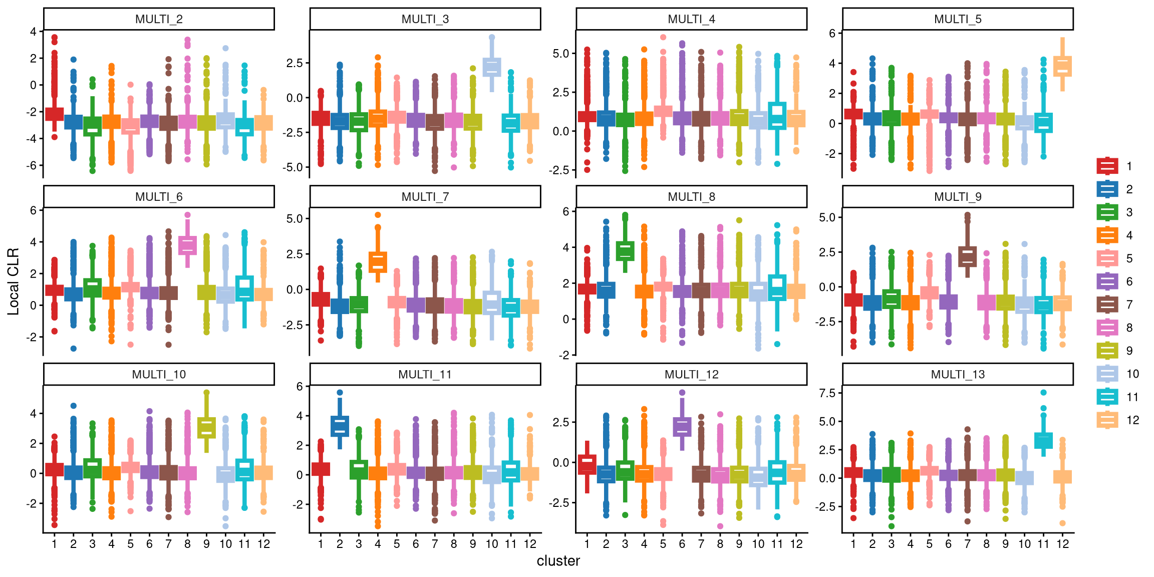
From the plot above, neither MULTI_2 nor MULTI_4 has a distinct box. Therefore, 12 clusters may not be appropriate for this dataset. We should then consider the optional workflow. A common approach is to add one more cluster.
In the updated clustering workflow, the optional parameter is set to TRUE, which enables the optional step for adding extra clusters. The extra_cluster parameter specifies the number of additional clusters to include. Here, we start by adding one extra cluster.
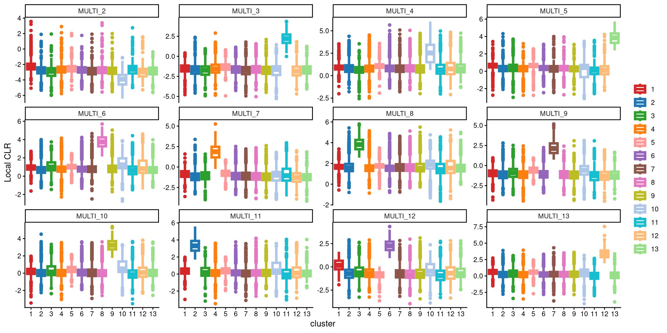
It is clear that the performance of MULTI_4 with 13 clusters is better than with 12 clusters. With 13 clusters, the box for cluster 10 is significantly higher than the other boxes. Therefore, 13 clusters appear to be a better choice.
Aside from the visualization check, we also provide a function that checks the CLR differences between the medians of the largest boxes in cases with fewer and more clusters for each hash label. The default threshold is set to 1. If the CLR difference for the more clustered case exceeds this threshold, we choose to use more clusters; otherwise, we use the default number of clusters, which remains unchanged.
## [1] "The largest CLR difference is:MULTI_4 1.268. Choose optional clustering method (kmed.cl2 with13 clusters)."For example, in MULTI_3, the largest box with 12 clusters corresponds to cluster 10, while with 13 clusters, it corresponds to cluster 11. The CLR difference between these two boxes is quite small, less than 1. In contrast, for MULTI_4, the largest box with 12 clusters is cluster 11, while with 13 clusters, it is cluster 10. The median CLR difference between these two boxes is significantly larger, exceeding 1.
We computed 12 pairs of median CLR differences for all 12 LMO labels, with the largest difference observed in MULTI_4, which exceeds 1. Therefore, we conclude that using 13 clusters provides better separation of the 12 LMO labels.
Next, the Euclidean distance between cells and their corresponding cluster centroid within each cluster is calculated using EuclideanClusterDist.
7.3 Definition of non-core cells
Core cells are defined as cells that are closer to their cluster centroids, while non-core cells are those that are farther away from the cluster centroid. The cut-off between core and non-core cells can be determined using EuclideanDistPlot, which visualizes the cut-off based on the quantile of the distribution via the eu_cut_q parameter, shown as the red line in the plot. Each value in the eu_cut_q parameter corresponds to a cut-off for a cluster.
EuclideanDistPlot(emlmo.cl.dist, eu_cut_q = c(0.9, 0.83, 0.65, 0.87, 0.91, 0.94, 0.8, 0.89, 0.84, 0.53, 0.9, 0.87, 0.88))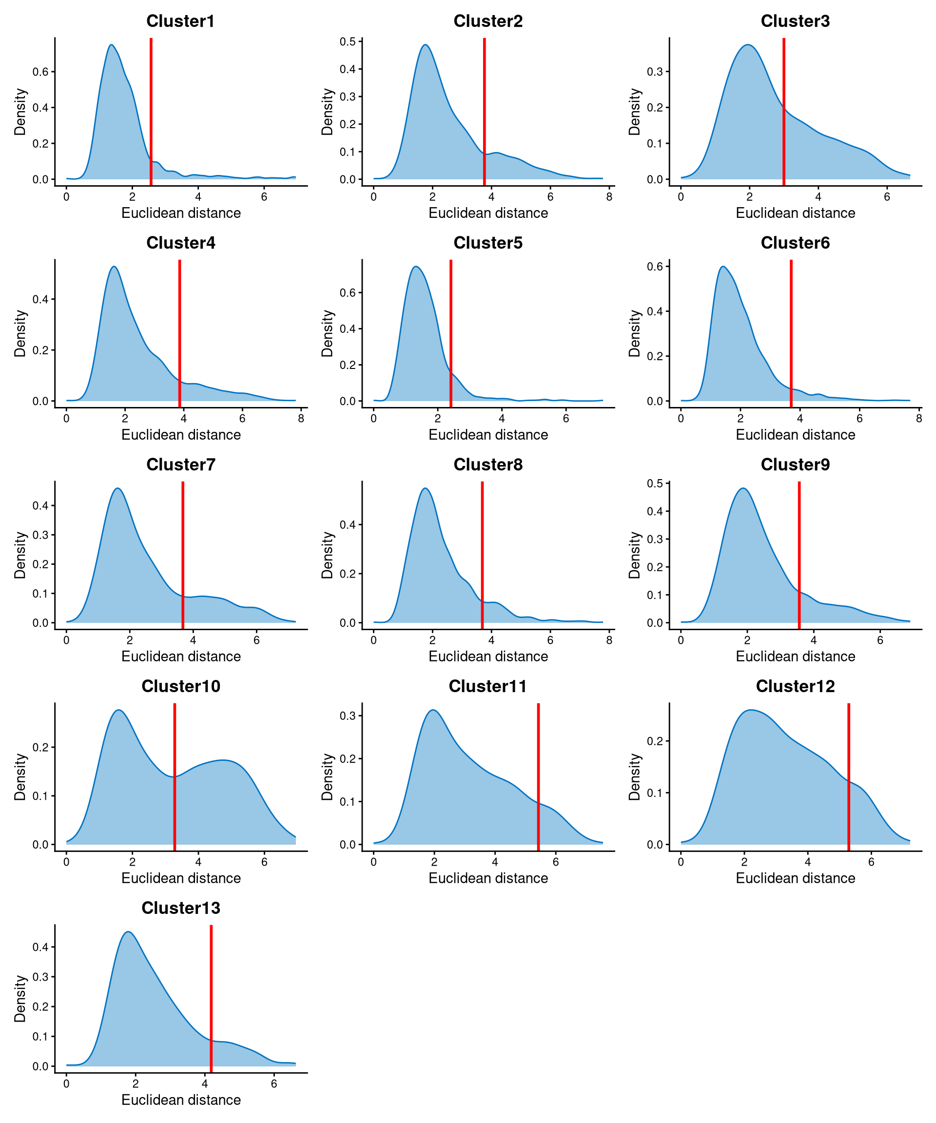
For most clusters, the Euclidean distances are right-skewed, and the cut-offs are selected at the tail of the distribution. For some clusters, such as clusters 2, 7, 8, and 10, the distances are bimodally distributed, so the cut-offs are selected at the anti-mode of the distribution. Cells with Euclidean distances larger than the cut-off are defined as non-core cells, while the remaining cells are defined as core cells.
Core and non-core cells are then classified using DefineNonCore, with eu_cut_q determined from the above plots. Since an optional extra cluster was added during the k-medoids clustering step, the optional parameter should be set to TRUE, and clr.norm should be supplied from the output of LocalCLRNorm.
emlmo.noncore <- DefineNonCore(emlmo.cl.dist, emlmo.kmed.cl2, eu_cut_q = c(0.9, 0.83, 0.65, 0.87, 0.91, 0.94, 0.8, 0.89, 0.84, 0.53, 0.9, 0.87, 0.88), optional = TRUE, clr.norm = emlmo.clr.norm)
table(emlmo.noncore)
## emlmo.noncore
## Cluster1 Cluster10 Cluster11 Cluster12 Cluster13 Cluster2 Cluster3 Cluster4 Cluster6 Cluster7 Cluster8 Cluster9 non-core
## 844 312 366 266 309 599 251 876 1452 562 858 649 2401Core cells are labelled by their clusters, and non-core cells are directly labelled as “non-core.”
The definition of core and non-core cells is further examined using CLRPlot.
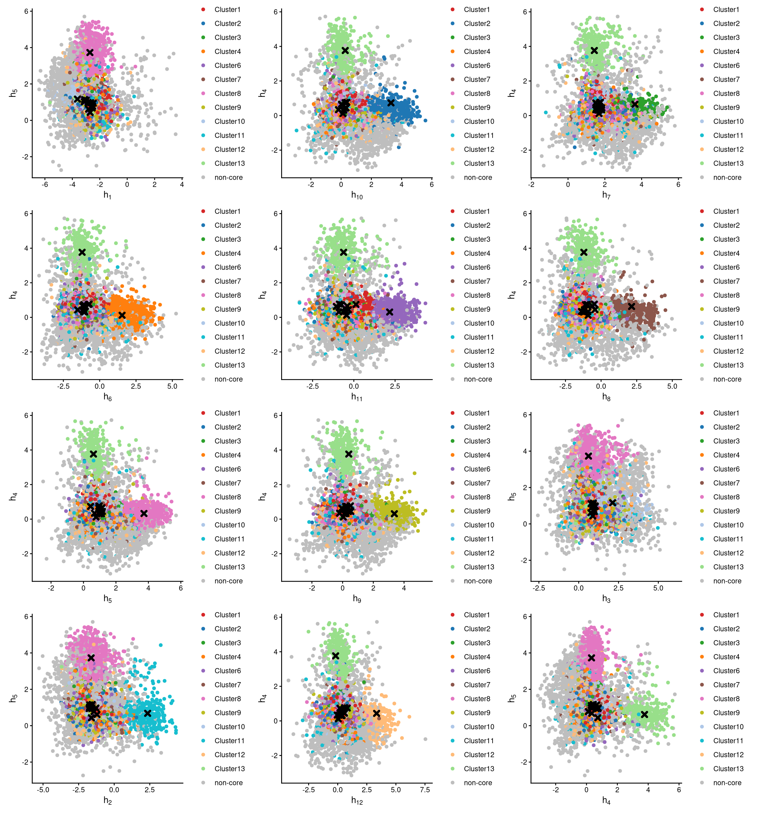
The pairwise local CLR-normalized values are shown in the above plots. Each plot clearly demonstrates two clusters, with other clusters appearing in the corners. Cluster centroids are indicated by cross symbols. These plots provide two important pieces of information:
All cells in cluster 5 are defined as non-core cells. Because one extra cluster was added during clustering, there should be exactly one cluster of cells defined as non-core.
MULTI_2 is not well assigned to any cluster. According to the
CheckCLRBoxPlot, MULTI_2 should theoretically correspond to cluster 1, as cluster 1 has the highest median local CLR value. However, in theCheckCLRBoxPlot, the expression of MULTI_2 in cluster 1 does not differ markedly from that in other clusters. In the pairwise CLR plot, the first plot also fails to show cluster 1 clearly, further indicating that MULTI_2 does not adequately label any cluster of cells.
7.4 Label clusters by sample
Each cluster will be labelled with its original sample, and here we use the default medoid-based labelling method.
emlmo.cluster.assign <- LabelClusterHTO(emlmo.clr.norm, emlmo.kmed.cl2, emlmo.noncore, label_method = "medoids")
emlmo.cluster.assign
## MULTI_2 MULTI_3 MULTI_4 MULTI_5 MULTI_6 MULTI_7 MULTI_8 MULTI_9 MULTI_10 MULTI_11 MULTI_12 MULTI_13
## 1 11 10 13 8 4 3 7 9 2 6 12The results show each sample and its corresponding cluster index. For example, cluster 1 corresponds to the MULTI_2 sample. Cluster 5 does not correspond to any sample, and its cells are non-core cells.
7.5 Computing the Mahalanobis distance
Using the local CLR-normalized values from LocalCLRNorm, the non-core cell classifications from DefineNonCore, the k-medoids clustering from KmedCluster, and the cluster labelling from LabelClusterHTO, the Mahalanobis distance for each single cell can be calculated using CalculateMD.
emlmo.md.mat <- CalculateMD(emlmo.clr.norm, emlmo.noncore, emlmo.kmed.cl2, emlmo.cluster.assign)
emlmo.md.mat[,1:10]
## AAACCCAAGAACTGAT-1 AAACCCAAGATGAAGG-1 AAACCCAAGGGTCTTT-1 AAACCCAAGTTGAAGT-1 AAACCCACAGAGTTCT-1 AAACCCACATAATGAG-1
## MULTI_2 3.013062 3.823441 5.053014 5.468070 2.273878 10.705157
## MULTI_3 5.940373 7.492579 8.408204 8.781191 4.907094 12.271943
## MULTI_4 3.932202 4.756061 5.034468 6.551176 2.584030 10.525790
## MULTI_5 7.614638 7.862808 9.236780 9.254290 6.665260 13.067936
## MULTI_6 5.757862 6.578008 7.374706 7.574423 4.914075 10.169824
## MULTI_7 4.155681 4.603995 6.954787 2.488210 3.841393 11.497299
## MULTI_8 5.240472 6.071785 3.416031 6.656167 4.025104 11.692990
## MULTI_9 5.943704 5.839436 6.479675 6.756596 4.169984 11.051626
## MULTI_10 3.269137 6.977949 7.208376 7.906082 4.593492 8.994215
## MULTI_11 6.306832 2.485724 8.229655 7.377072 5.711002 8.208022
## MULTI_12 4.112570 5.142894 6.311139 6.723983 4.540724 11.173421
## MULTI_13 6.207978 6.512022 4.997592 8.555328 5.606367 12.169857
## AAACCCAGTACTAGCT-1 AAACCCAGTCGTAATC-1 AAACCCAGTGTGATGG-1 AAACCCATCAGATGCT-1
## MULTI_2 1.950891 6.613351 4.629565 2.925876
## MULTI_3 7.394122 8.688644 7.779191 7.220167
## MULTI_4 3.534758 7.260183 6.421863 4.266364
## MULTI_5 6.944218 11.158016 9.000311 7.204465
## MULTI_6 5.377147 8.092866 6.625383 4.159365
## MULTI_7 5.420922 5.532282 6.769361 5.882408
## MULTI_8 4.220768 5.123240 6.866812 4.074846
## MULTI_9 5.520278 8.493584 7.053675 5.313671
## MULTI_10 5.405723 9.026629 7.802017 6.331922
## MULTI_11 5.991758 8.541005 7.339129 5.785192
## MULTI_12 3.146046 7.639954 3.999722 4.967005
## MULTI_13 4.590890 8.681299 7.395827 5.058285The output is a Mahalanobis distance matrix with rows representing hashtag samples and columns representing cells. Each entry indicates the Mahalanobis distance of a cell to a given hashtag sample.
7.6 Detect outlier cells
Outlier cells, including negatives and doublets, are defined based on the distribution of the minimum Mahalanobis distance across all cells, which can be visualized using MDDensPlot. The cut-off in the plot is determined by the md_cut_q parameter, which specifies the quantile of the distribution and is shown as the red line. Users are encouraged to adjust the cut-off through the md_cut_q parameter.
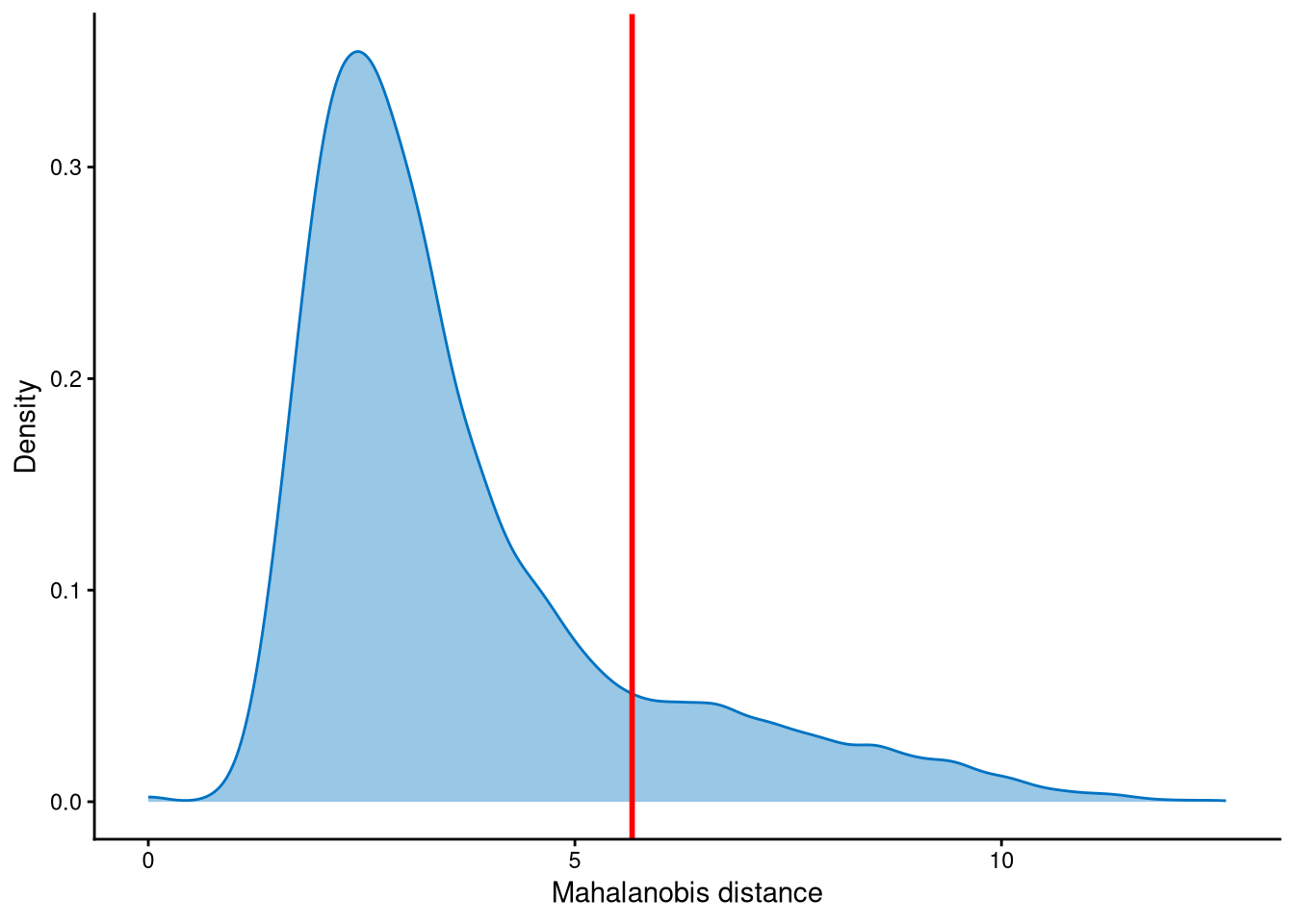
The distribution of Mahalanobis distance is likely to be bimodally distributed, and the cut-off can be set at the anti-mode position of the distribution. Cells with Mahalanobis distance larger than the cut-off are defined as outlier cells, and other cells are singlets.
Outlier cells are then defined using AssignOutlierDrop according to the cut-off selected from the plot.
emlmo.outlier.assign <- AssignOutlierDrop(emlmo.md.mat, md_cut_q = 0.85)
table(emlmo.outlier.assign)
## emlmo.outlier.assign
## Outlier Singlet
## 1462 8283In this step, cells are labelled as either outliers or singlets.
7.7 Demultiplexing
The HTO library sizes are used to further distinguish negatives and doublets among the outlier cells. The distribution of HTO library sizes can be visualized using OutlierHTOPlot. The possible cut-offs corresponding to the modes and anti-modes are shown as red lines in the plot. The parameter num_modes is used to set the number of modes in the plot.
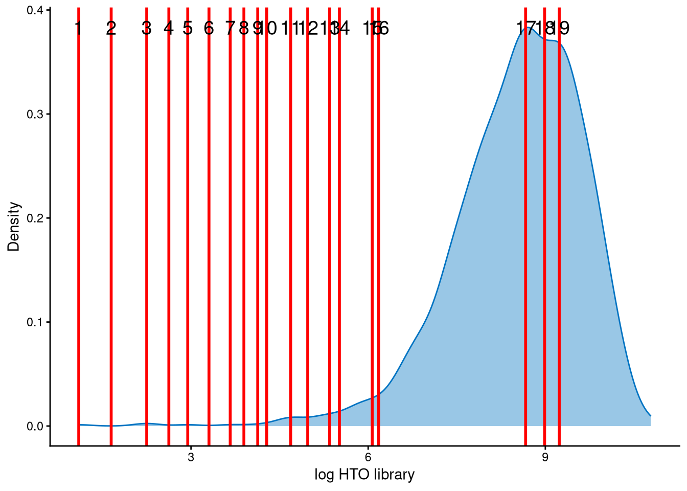
The distribution of HTO library sizes for these outlier cells is not typically multimodal; instead, it is left-skewed. The 19 lines represent possible cut-offs used to distinguish negatives from doublets. These lines indicate all modes and anti-modes. Line 12 is an appropriate cut-off for separating negatives from doublets, and the corresponding HTO library size (total hashtag counts per cell) is approximately \(e^5\approx148\), which is a reasonable threshold.
In the final step of demultiplexing, the Mahalanobis distance from CalculateMD, the original hashtag count matrix, the outlier classifications from AssignOutlierDrop, the gene expression data, and the selected HTO library size cut-off from the above plot are applied. In addition, since optional extra clusters were generated for this dataset, the parameter optional should be set to TRUE. kmed.cl should be provided from the output of KmedCluster, and clr.norm from the output of LocalCLRNorm. The remaining three parameters, unlabel_cl_cut, unlabel_raw_cut, and unlabel_clr_cut, relate to the cut-offs for the unlabelled hash (in this dataset, MULTI_2). Because unlabelled hashes are rare, we recommend using the default values and modifying these three parameters only if necessary.
emlmo.cmddemux.assign <- CMDdemuxClass(emlmo.md.mat, emlmo.hash.count, emlmo.outlier.assign, use_gex_data = TRUE, gex.count = emlmo.gex.count,  num_modes = 10, cut_no = 12, optional = TRUE, kmed.cl = emlmo.kmed.cl2,  clr.norm = emlmo.clr.norm, unlabel_cl_cut = 0.5, unlabel_raw_cut = 4.6, unlabel_clr_cut = -0.5)
head(emlmo.cmddemux.assign)
## demux_id global_class demux_global_class doublet_class
## AAACCCAAGAACTGAT-1 MULTI_2 Negative Negative Negative
## AAACCCAAGATGAAGG-1 MULTI_11 Singlet MULTI_11 MULTI_11
## AAACCCAAGGGTCTTT-1 MULTI_8 Singlet MULTI_8 MULTI_8
## AAACCCAAGTTGAAGT-1 MULTI_7 Singlet MULTI_7 MULTI_7
## AAACCCACAGAGTTCT-1 MULTI_2 Negative Negative Negative
## AAACCCACATAATGAG-1 MULTI_11 Singlet MULTI_11 MULTI_11CMDdemux provides four types of outputs:
demux_id: the identity for each cell, determined by the sample with the minimum Mahalanobis distance for that cell.
global_class: classification of each cell as Singlet, Doublet, or Negative.
demux_global_class: singlet cells are labeled with their original sample, while negatives and doublets are labeled accordingly.
doublet_class: similar to demux_global_class, but doublets are labeled with their sample of origin. This is particularly useful for combined-hashtag experiments.
##
##  Doublet MULTI_10 MULTI_11 MULTI_12 MULTI_13  MULTI_2  MULTI_3  MULTI_4  MULTI_5  MULTI_6  MULTI_7  MULTI_8  MULTI_9 Negative
##      699      747      686     1464      275        6      330      536      356      950      925      372      658     1741
The output above shows the number of cells demultiplexed into each category.
The interpretations of unlabel_cl_cut, unlabel_raw_cut, and unlabel_clr_cut are as follows:
unlabel_cl_cut corresponds to the difference in local CLR values between the top two clusters (i.e., the clusters with the highest and second-highest local CLR values). If a hashtag has a difference smaller than unlabel_cl_cut, it is considered an unlabelled hash. For example, referring to the CheckCLRBoxPlot for the 13-cluster version, clusters 1 and 5 have the top two median CLR values for MULTI_2, and their median difference is smaller than the default value 0.5. Therefore, MULTI_2 should be considered an unlabelled hash.
After determining that the dataset contains an unlabelled hash, the cells initially classified as negatives are further examined. For each negative cell, its log raw HTO count for the unlabelled hash (MULTI_2 in this dataset) is compared with the cut-off defined by unlabel_raw_cut, and the difference between the local CLR value of the unlabelled hash and the maximum local CLR value in that cell is calculated and compared with unlabel_clr_cut. Cells with values exceeding both cut-offs are rescued as singlets belonging to MULTI_2. The underlying rationale is that singlets belonging to the unlabelled hash should have high raw expression of the unlabelled hash, and its CLR-normalized value should be the highest within the cell. This is described in Supplementary Methods Section S4 and illustrated in Fig. S2b.
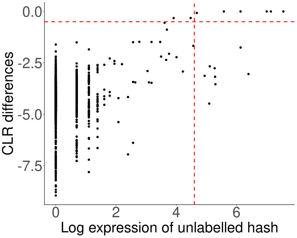
Figure 7.1: Rescue MULTI_2 singlets.
The horizontal red line corresponds to unlabel_clr_cut, and the vertical red line corresponds to unlabel_raw_cut. Cells located above both cut-offs (i.e., in the upper-right quadrant) are rescued as MULTI_2 singlets.
7.8 Examination of suspicious droplets
In our CMDdemux paper, we identified that the major differences between CMDdemux and HTODemux are that HTODemux assigns more doublets than CMDdemux, whereas CMDdemux assigns more MULTI_4 singlets. We can use CheckAssign2DPlot and CheckAssign3DPlot to visually verify whether the CMDdemux results are correct.
CheckAssign2DPlot consists of pairwise 2D plots of HTO library sizes, mRNA library sizes, the second Mahalanobis distance, and the ratio of the first to the second Mahalanobis distance. Negatives, singlets, and doublets are separated into different regions in these 2D plots.
CheckAssign3DPlot uses HTO library sizes, mRNA library sizes, and the ratio of the first to the second Mahalanobis distance to visualize negatives, singlets, and doublets in 3D.
First, we apply HTODemux to this dataset.
library(Seurat)
emlmo.obj <- CreateSeuratObject(counts = emlmo.hash.count)
emlmo.obj[["HTO"]] <- CreateAssayObject(counts = emlmo.hash.count)
emlmo.obj <- NormalizeData(emlmo.obj, assay = "HTO", normalization.method = "CLR")
emlmo.obj <- HTODemux(emlmo.obj, assay = "HTO", positive.quantile = 0.99)
We then randomly select 30 cells that are assigned as MULTI_4 singlets by CMDdemux but as doublets or negatives by HTODemux.
emlmo.extra.multi4 <- intersect(rownames(emlmo.cmddemux.assign)[which(emlmo.cmddemux.assign$demux_global_class == "MULTI_4")], names(emlmo.obj$HTO_classification.global)[which(emlmo.obj$HTO_classification.global %in% c("Negative", "Doublet"))])
set.seed(2026)
barcode.random.idx1 <- sample(1:length(emlmo.extra.multi4), 30, replace = FALSE)
Next, we use CheckAssign2DPlot to examine these 30 cells.
CheckAssign2DPlot(emlmo.hash.count, emlmo.gex.count, emlmo.md.mat, cmddemux.assign = emlmo.cmddemux.assign, check_barcodes = emlmo.extra.multi4[barcode.random.idx1], check_barcode_size = 3)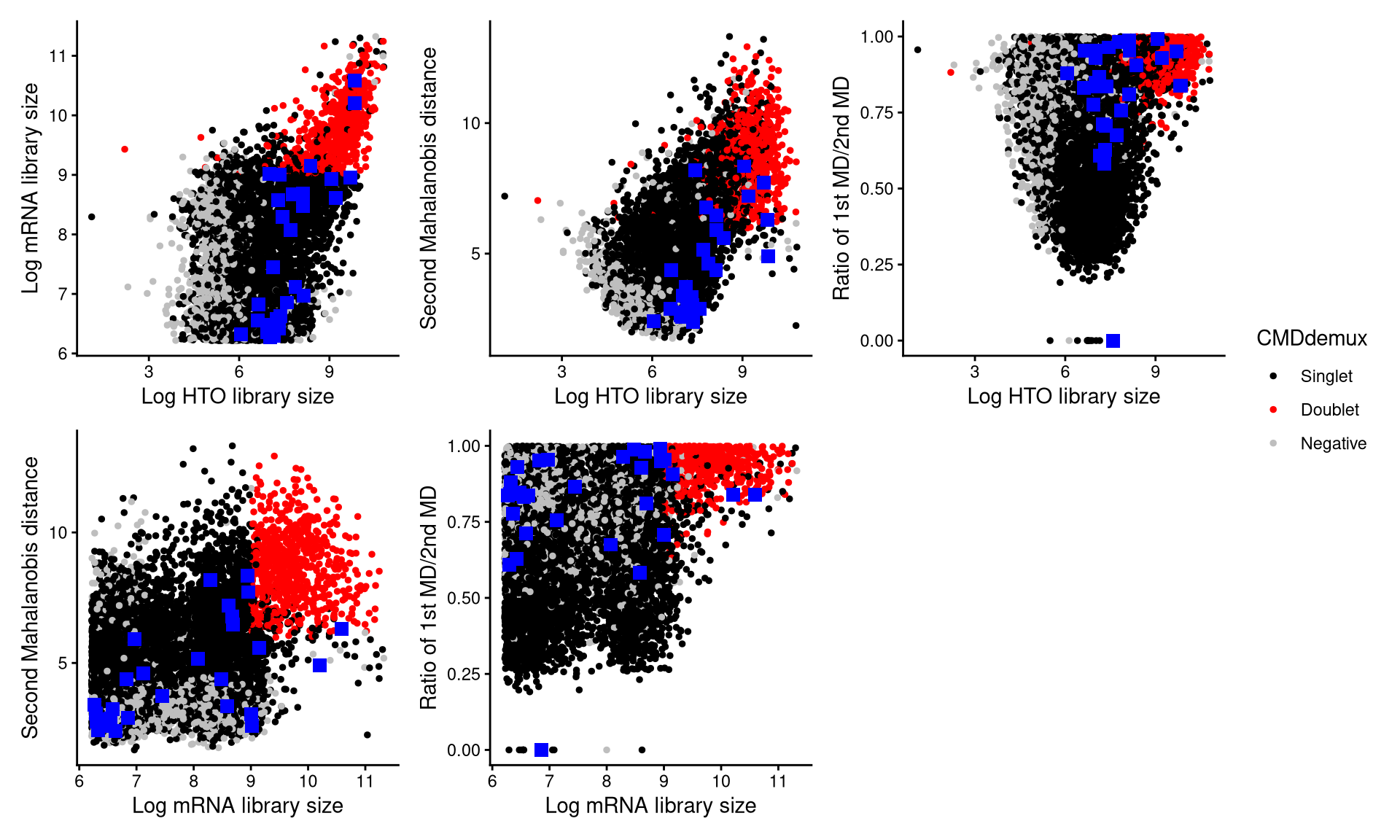
The randomly selected cells are shown as blue squares. Most of them fall within the singlet region, indicating that they should be classified as singlets.
These cells can also be visualized using CheckAssign3DPlot.
CheckAssign3DPlot(emlmo.hash.count, emlmo.gex.count, emlmo.md.mat, cmddemux.assign = emlmo.cmddemux.assign, check_barcodes = emlmo.extra.multi4[barcode.random.idx1])In the 3D plot, the 30 randomly selected cells are shown as blue points, and most are again located in the singlet region, further supporting the CMDdemux assignments.
We then examine droplets assigned as doublets by HTODemux but as singlets by CMDdemux.
Thirty such cell barcodes are randomly selected, as shown below.
emlmo.extra.doublet <- intersect(rownames(emlmo.cmddemux.assign)[which(emlmo.cmddemux.assign$global_class == "Singlet")], names(emlmo.obj$HTO_classification.global)[which(emlmo.obj$HTO_classification.global == "Doublet")])
set.seed(2026)
barcode.random.idx2 <- sample(1:length(emlmo.extra.doublet), 30, replace = FALSE)CheckAssign2DPlot(emlmo.hash.count, emlmo.gex.count, emlmo.md.mat, cmddemux.assign = emlmo.cmddemux.assign, check_barcodes = emlmo.extra.doublet[barcode.random.idx2], check_barcodes_col = "green", check_barcode_size = 3)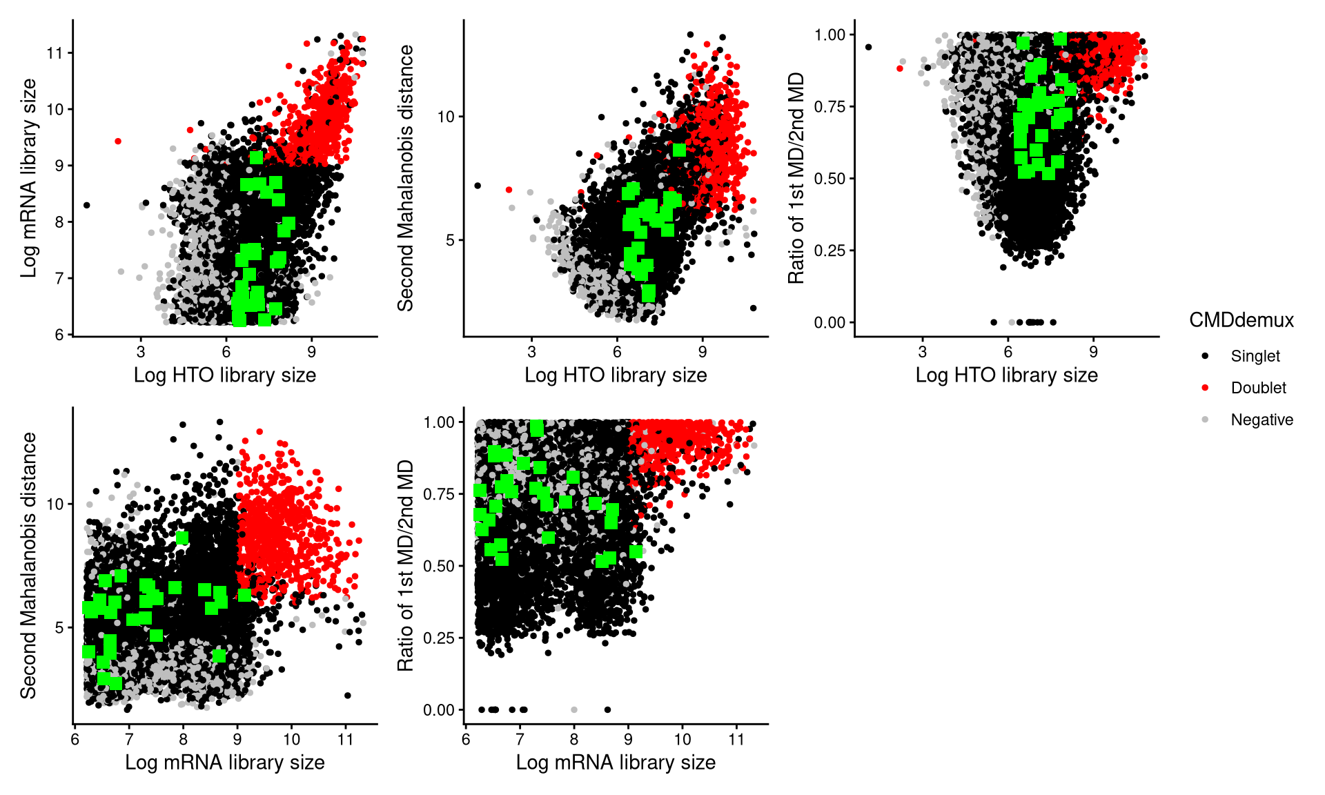
Using CheckAssign2DPlot, the selected cells appear as green squares in the plots. Most lie in the singlet region, suggesting that they should be demultiplexed as singlets.
CheckAssign3DPlot provides a similar visualization.
CheckAssign3DPlot(emlmo.hash.count, emlmo.gex.count, emlmo.md.mat, cmddemux.assign = emlmo.cmddemux.assign, check_barcodes = emlmo.extra.doublet[barcode.random.idx2], check_barcodes_col = "green")In the 3D plot, the 30 cells appear as green points and largely overlap with the singlet population, further supporting that these droplets should be classified as singlets rather than doublets, thereby validating the CMDdemux results.