Chapter 10 PDX Hashtag Ab
This dataset is low quality (Brown et al. 2024) and contains 7,071 cells derived from a human ovarian carcinosarcoma patient-derived xenograft (PDX). Nuclei from four donors were labelled using TotalSeqTM-A anti–nuclear pore complex antibodies. The low quality is due to the low input, and the whole-cell hashing data exhibit weak signals.
The subset of hash count data is shown below:
## 4 x 10 sparse Matrix of class "dgCMatrix"## [[ suppressing 10 column names 'AAACCCAAGCCATTGT-1', 'AAACCCACAAAGGGTC-1', 'AAACCCACACCTTCGT-1' ... ]]##
## CMO301 183 525 315 159 40 55 33 209 94 108
## CMO302 42 155 76 185 365 17 14 26 328 113
## CMO303 35 31 64 18 9 10 8 13 6 13
## CMO304 29 158 57 35 6 241 103 122 5 10The subset of gene expression data is shown below:
## 10 x 10 sparse Matrix of class "dgCMatrix"## [[ suppressing 10 column names 'AAACCCAAGCCATTGT-1', 'AAACCCACAAAGGGTC-1', 'AAACCCACACCTTCGT-1' ... ]]##
## AL627309.1 . . . . . . . . . .
## AL627309.5 . . . . . . . . . .
## AL627309.4 . . . . . . . . . .
## AC114498.1 . . . . . . . . . .
## AL669831.2 . . . . . . . . . .
## LINC01409 . . . . . . . . . .
## FAM87B . . . . . . . . . .
## LINC01128 . . . . . . . . . .
## LINC00115 . . . . . . . . . .
## AL645608.6 . . . . . . . . . .10.1 Local CLR normalization
The first step of CMDdemux is to normalize the hash count data using a local CLR normalization.
##       AAACCCAAGACCATGG-1 AAACCCAAGGGTCTTT-1 AAACCCACACAATGAA-1 AAACCCACACTTTAGG-1 AAACCCACATTAGGCT-1 AAACCCAGTTCCCAAA-1
## HTO_1        0.841950893          0.7052793          0.7036046          0.9942375          0.8073046         1.10630286
## HTO_2       -0.049022031          0.0818120         -0.1465463          0.2455204         -0.1676937        -0.01762724
## HTO_3       -0.784728826         -0.9249927         -0.6573720         -1.3639175         -0.4949066        -0.83337674
## HTO_4       -0.008200036          0.1379015          0.1003137          0.1241596         -0.1447042        -0.25529889
##       AAACCCAGTTGCCATA-1 AAACCCAGTTGCCTAA-1 AAACCCAGTTTCACAG-1 AAACCCATCATGCAGT-1
## HTO_1          0.7632379          1.4016463         1.87616197          1.3115176
## HTO_2          0.1213840          0.4012724        -0.05949168          0.1022954
## HTO_3         -0.9916171         -0.6460466        -0.96394796         -0.8052616
## HTO_4          0.1069952         -1.1568722        -0.85272232         -0.6085513
The output of LocalCLRNorm is a normalized data matrix with rows representing hashtag samples and columns representing cells. Each entry is a normalized value.
10.2 K-medoids clustering
The local CLR-normalized values are used here for K-medoids clustering. Since this dataset has four samples, the default parameters are initially applied, which divide the cells into four clusters.
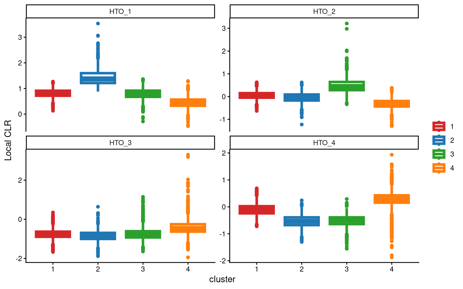
For HTO_3, the differences among the four clusters are not significant. Therefore, we should try using more clusters.
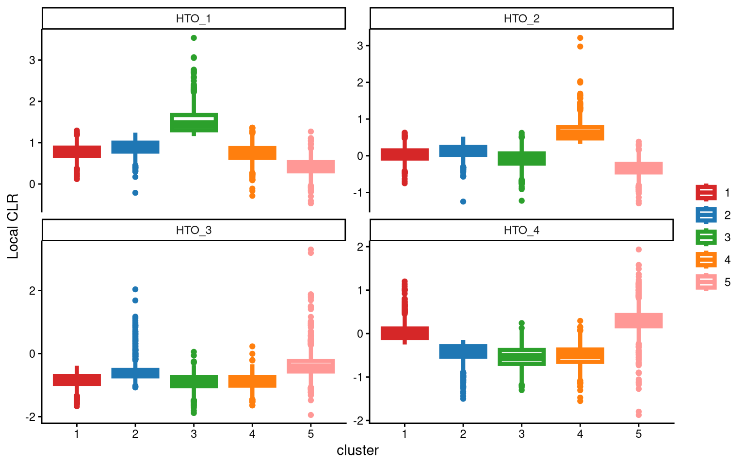
For HTO_3, we still do not get an ideal separation of clusters. Try adding one more cluster. In the function KmedCluster, the extra_cluster parameter specifies the number of clusters used in clustering.
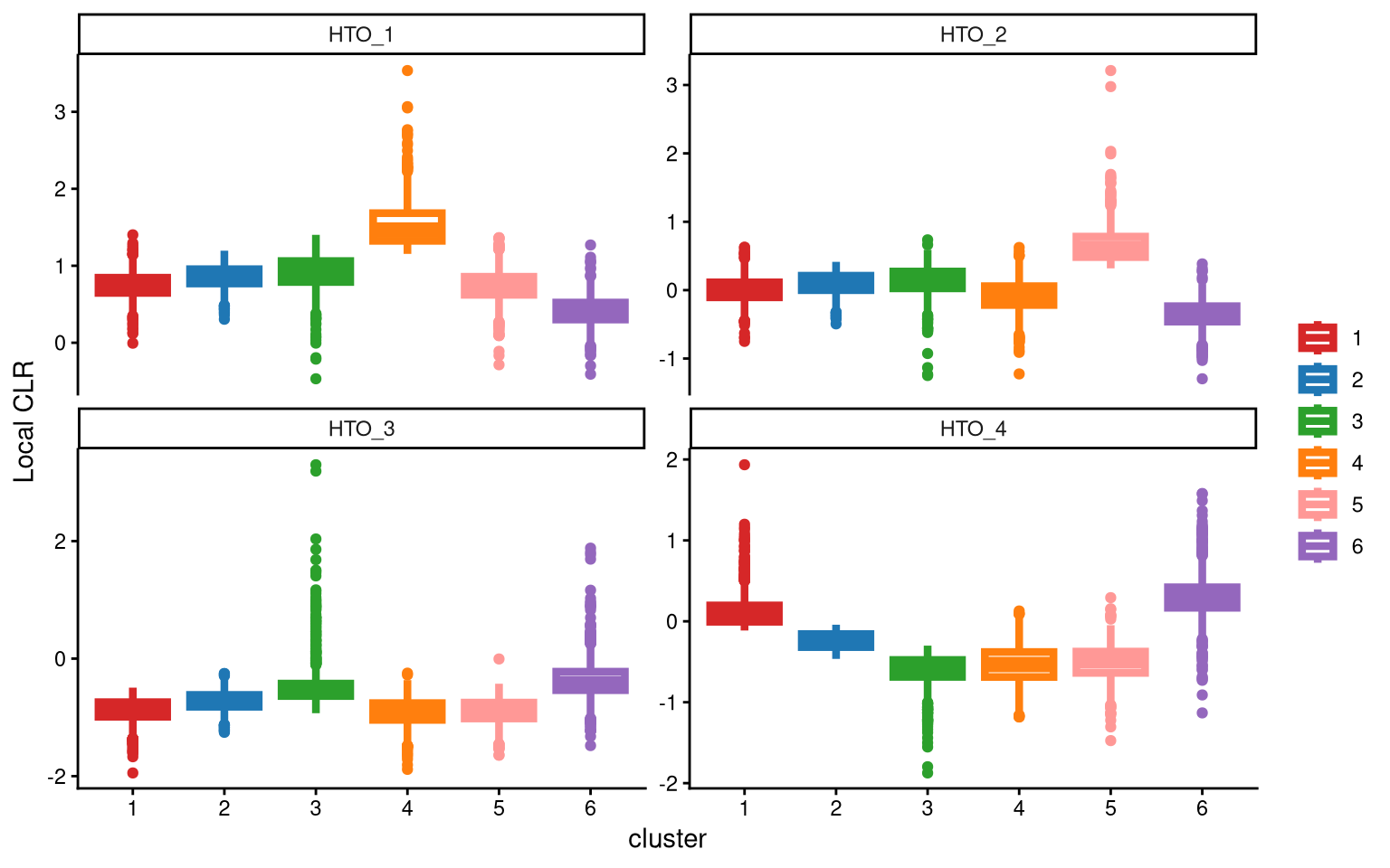
For HTO_3, we still do not obtain an ideal cluster with significantly higher expression compared to other clusters. Therefore, we choose to add one more cluster.
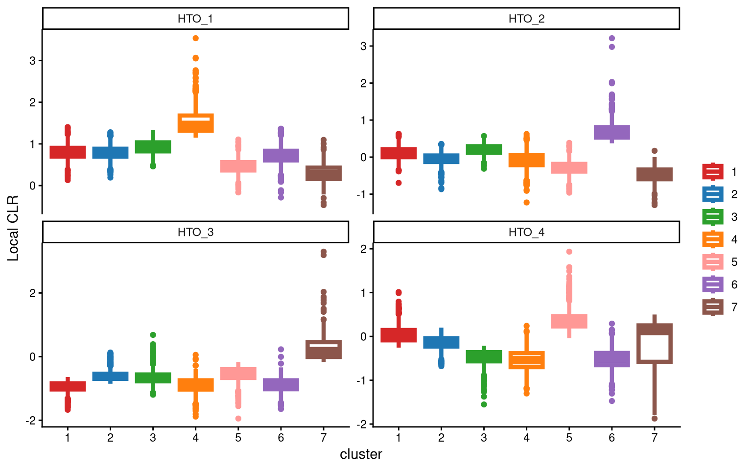
This time, we obtain cluster 7 in HTO_3 with higher expression compared to all other clusters. Therefore, seven clusters are ideal for this PDX HTO data.
Next, the function ExamineClusterNumber is used again to check the number of clusters in the data. From the plot, we observe that the CLR differences between the top two clusters are less than 1 for all hashtags. Therefore, fc_cut is set to a smaller value of 0.5 instead of the default, as this dataset is special.
## [1] "The largest CLR difference is:HTO_3 0.644. Choose optional clustering method (kmed.cl2 with7 clusters)."The function confirms that seven clusters are appropriate for this data.
Next, the Euclidean distance between cells and their corresponding cluster centroid within each cluster is calculated using EuclideanClusterDist.
10.3 Definition of non-core cells
Core cells are defined as cells that are closer to their cluster centroids, while non-core cells are those that are farther away from the cluster centroid. The cut-off between core and non-core cells can be determined using EuclideanDistPlot, which visualizes the cut-off based on the quantile of the distribution via the eu_cut_q parameter, shown as the red line in the plot. Each value in the eu_cut_q parameter corresponds to a cut-off for a cluster.
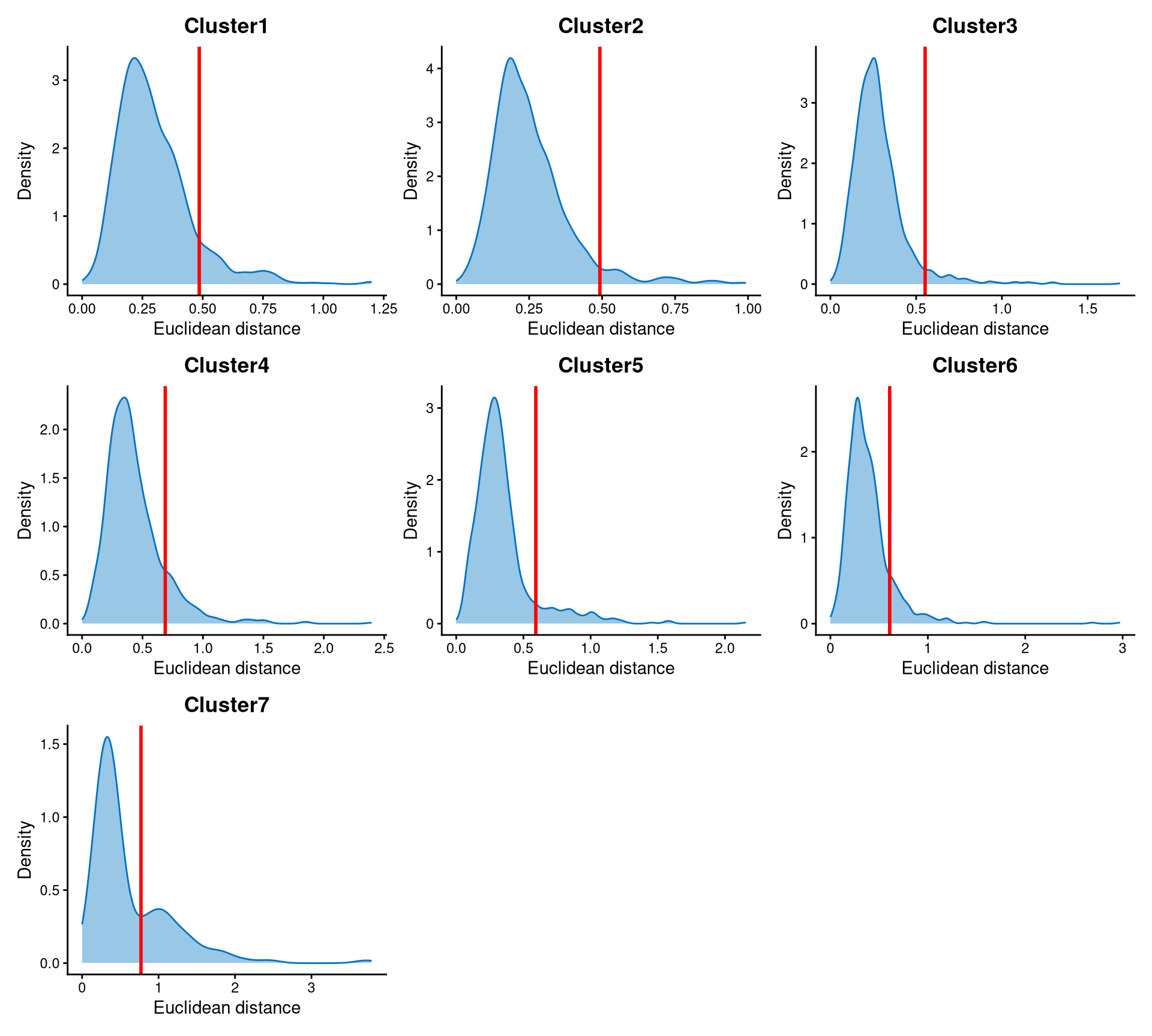
For most clusters, the distribution of Euclidean distances is right-skewed, and the cut-off is set at the tail of the distribution. For cluster 7, the Euclidean distances are bimodally distributed, and the cut-off is set at the anti-mode of the distribution.
Core and non-core cells are then classified using DefineNonCore, with eu_cut_q determined from the above plots. Since three optional extra clusters were added during the k-medoids clustering step, the optional parameter should be set to TRUE, and clr.norm should be supplied from the output of LocalCLRNorm.
pdxhto.noncore <- DefineNonCore(pdxhto.cl.dist, pdxhto.kmed.cl4, eu_cut_q = c(0.9, 0.95, 0.95, 0.88, 0.9, 0.88, 0.71), optional = TRUE, clr.norm = pdxhto.clr.norm)
table(pdxhto.noncore)
## pdxhto.noncore
## Cluster4 Cluster5 Cluster6 Cluster7 non-core
## 889 837 785 209 4351Core cells are labelled by their clusters, and non-core cells are directly labelled as “non-core.”
The definition of core and non-core cells is further examined using CLRPlot.
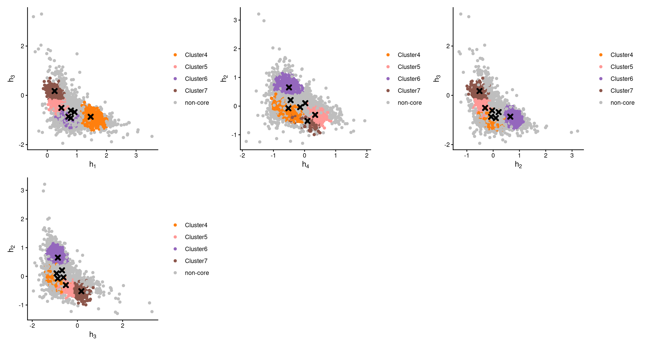
The pairwise local CLR-normalized values are shown in the above plots. Each plot clearly demonstrates two clusters, with other clusters appearing in the corners. Cluster centroids are indicated by cross symbols. All cells in cluster 1,2 and 3 are defined as non-core cells. Because three extra clusters were added during clustering, there should be exactly three clusters of cells defined as non-core. However, cluster 1, 2 and 3 are not uniquely or highly expressing any hashtag in the CheckCLRBoxPlot for the version with 7 clusters.
10.4 Label clusters by sample
Each cluster will be labelled with its original sample, and here we use the alternative labelling method, “expression”. Each hashtag sample is assigned to the cluster has the maximum median local CLR value.
pdxhto.cluster.assign <- LabelClusterHTO(pdxhto.clr.norm, pdxhto.kmed.cl4, pdxhto.noncore, label_method = "expression")
pdxhto.cluster.assign
## HTO_1 HTO_2 HTO_3 HTO_4
## 4 6 7 5The results show each sample and its corresponding cluster index. For example, cluster 4 corresponds to the HTO_1 sample. Cluster 1, 2, and 3 do not correspond to any sample, and their cells are non-core cells.
10.5 Computing the Mahalanobis distance
Using the local CLR-normalized values from LocalCLRNorm, the non-core cell classifications from DefineNonCore, the k-medoids clustering from KmedCluster, and the cluster labelling from LabelClusterHTO, the Mahalanobis distance for each single cell can be calculated using CalculateMD.
pdxhto.md.mat <- CalculateMD(pdxhto.clr.norm, pdxhto.noncore, pdxhto.kmed.cl4, pdxhto.cluster.assign)
pdxhto.md.mat[,1:10]
## AAACCCAAGACCATGG-1 AAACCCAAGGGTCTTT-1 AAACCCACACAATGAA-1 AAACCCACACTTTAGG-1 AAACCCACATTAGGCT-1 AAACCCAGTTCCCAAA-1
## HTO_1 3.998914 5.090501 4.914767 4.962751 4.109228 2.244173
## HTO_2 4.424295 4.218390 5.131412 4.515180 4.998319 4.288759
## HTO_3 5.838773 6.393968 4.841916 8.932623 4.629366 6.951389
## HTO_4 3.022285 3.132145 1.897709 5.563477 2.909380 4.664140
## AAACCCAGTTGCCATA-1 AAACCCAGTTGCCTAA-1 AAACCCAGTTTCACAG-1 AAACCCATCATGCAGT-1
## HTO_1 4.865596 4.035444 2.646610 1.334294
## HTO_2 4.017997 5.088924 7.368723 4.370025
## HTO_3 6.832309 10.120147 10.814867 8.257401
## HTO_4 3.594449 9.146110 9.288884 6.556850The output is a Mahalanobis distance matrix with rows representing hashtag samples and columns representing cells. Each entry indicates the Mahalanobis distance of a cell to a given hashtag sample.
10.6 Detect outlier cells
Outlier cells, including negatives and doublets, are defined based on the distribution of the minimum Mahalanobis distance across all cells, which can be visualized using MDDensPlot. The cut-off in the plot is determined by the md_cut_q parameter, which specifies the quantile of the distribution and is shown as the red line. Users are encouraged to adjust the cut-off through the md_cut_q parameter.
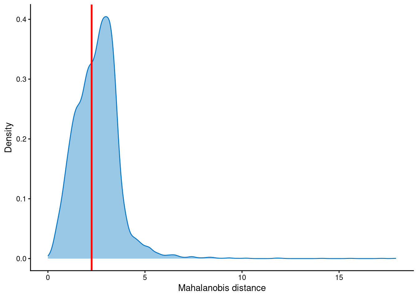
The distribution of Mahalanobis distances is right-skewed, and the cut-off is set at an anti-mode of the distribution.
Outlier cells are then defined using AssignOutlierDrop according to the cut-off selected from the plot.
pdxhto.outlier.assign <- AssignOutlierDrop(pdxhto.md.mat, md_cut_q = 0.4)
table(pdxhto.outlier.assign)
## pdxhto.outlier.assign
## Outlier Singlet
## 4242 2829In this step, cells are labelled as either outliers or singlets.
10.7 Demultiplexing
The HTO library sizes are used to further distinguish negatives and doublets among the outlier cells. The distribution of HTO library sizes can be visualized using OutlierHTOPlot. The possible cut-offs corresponding to the modes and anti-modes are shown as red lines in the plot. The parameter num_modes is used to set the number of modes in the plot.
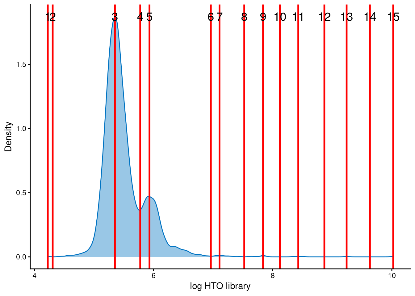
The HTO library sizes for these outlier cells are bimodally distributed, and line no. 4, at the anti-mode of this distribution, provides a reasonable cut-off to separate negatives and doublets among the outliers.
In the final step of demultiplexing, the Mahalanobis distance from CalculateMD, the original hashtag count matrix, the outlier classifications from AssignOutlierDrop, the gene expression data, and the selected HTO library size cut-off from the above plot are applied. Since optional clustering was applied to this dataset with extra clusters, optional is set to TRUE. K-medoids clustering from KmedCluster and the sample-label assignment from LabelClusterHTO are then applied to obtain the final demultiplexing results.
pdxhto.cmddemux.assign <- CMDdemuxClass(pdxhto.md.mat, pdxhto.hash.count, pdxhto.outlier.assign, use_gex_data = TRUE, gex.count = pdxhto.gex.count, num_modes = 8, cut_no = 4, optional = TRUE, kmed.cl = pdxhto.kmed.cl4, cluster.assign = pdxhto.cluster.assign)
head(pdxhto.cmddemux.assign)
## demux_id global_class demux_global_class doublet_class
## AAACCCAAGACCATGG-1 HTO_4 Negative Negative Negative
## AAACCCAAGGGTCTTT-1 HTO_4 Doublet Doublet HTO_2_HTO_4
## AAACCCACACAATGAA-1 HTO_4 Singlet HTO_4 HTO_4
## AAACCCACACTTTAGG-1 HTO_2 Singlet HTO_2 HTO_2
## AAACCCACATTAGGCT-1 HTO_4 Singlet HTO_4 HTO_4
## AAACCCAGTTCCCAAA-1 HTO_1 Singlet HTO_1 HTO_1CMDdemux provides four types of outputs:
demux_id: the identity for each cell, determined by the sample with the minimum Mahalanobis distance for that cell.
global_class: classification of each cell as Singlet, Doublet, or Negative.
demux_global_class: singlet cells are labeled with their original sample, while negatives and doublets are labeled accordingly.
doublet_class: similar to demux_global_class, but doublets are labeled with their sample of origin. This is particularly useful for combined-hashtag experiments.
##
##  Doublet    HTO_1    HTO_2    HTO_3    HTO_4 Negative
##      749     1098     1535      239     1634     1816
The output above shows the number of cells demultiplexed into each category.
10.8 Examination of suspicious droplets
In the original paper, HTODemux assigns more HTO_1 singlets, while CMDdemux demultiplexes those cells as doublets. Additionally, HTODemux assigns more doublets, whereas CMDdemux assigns more singlets in the HTO_3 and HTO_4 samples. We can use the functions CheckAssign2DPlot and CheckAssign3DPlot to visually assess whether the CMDdemux assignments are correct.
CheckAssign2DPlot consists of pairwise 2D plots of HTO library sizes, mRNA library sizes, the second Mahalanobis distance, and the ratio of the first to the second Mahalanobis distance. Negatives, singlets, and doublets are separated into different regions in these 2D plots.
CheckAssign3DPlot uses HTO library sizes, mRNA library sizes, and the ratio of the first to the second Mahalanobis distance to visualize negatives, singlets, and doublets in 3D.
First, apply HTODemux to the data.
pdxhto.obj <- CreateSeuratObject(counts = pdxhto.hash.count)
pdxhto.obj[["HTO"]] <- CreateAssayObject(counts = pdxhto.hash.count)
pdxhto.obj <- NormalizeData(pdxhto.obj, assay = "HTO", normalization.method = "CLR")
pdxhto.obj <- HTODemux(pdxhto.obj, assay = "HTO", positive.quantile = 0.95)
We then examine the cells that are assigned as doublets by CMDdemux but classified as HTO_1 singlets by HTODemux. For this examination, 30 cells are randomly selected from this group.
pdxhto.extra.doublet <- intersect(rownames(pdxhto.cmddemux.assign)[which(pdxhto.cmddemux.assign$demux_global_class == "Doublet")], names(pdxhto.obj$HTO_classification.global)[which(pdxhto.obj$hash.ID == "HTO-1")])
set.seed(2026)
barcode.random.idx1 <- sample(1:length(pdxhto.extra.doublet), 30, replace = FALSE)
We then use CheckAssign2DPlot to visualize these cells in 2D.
CheckAssign2DPlot(pdxhto.hash.count, pdxhto.gex.count, pdxhto.md.mat, cmddemux.assign = pdxhto.cmddemux.assign, check_barcodes = pdxhto.extra.doublet[barcode.random.idx1], check_barcode_size = 3)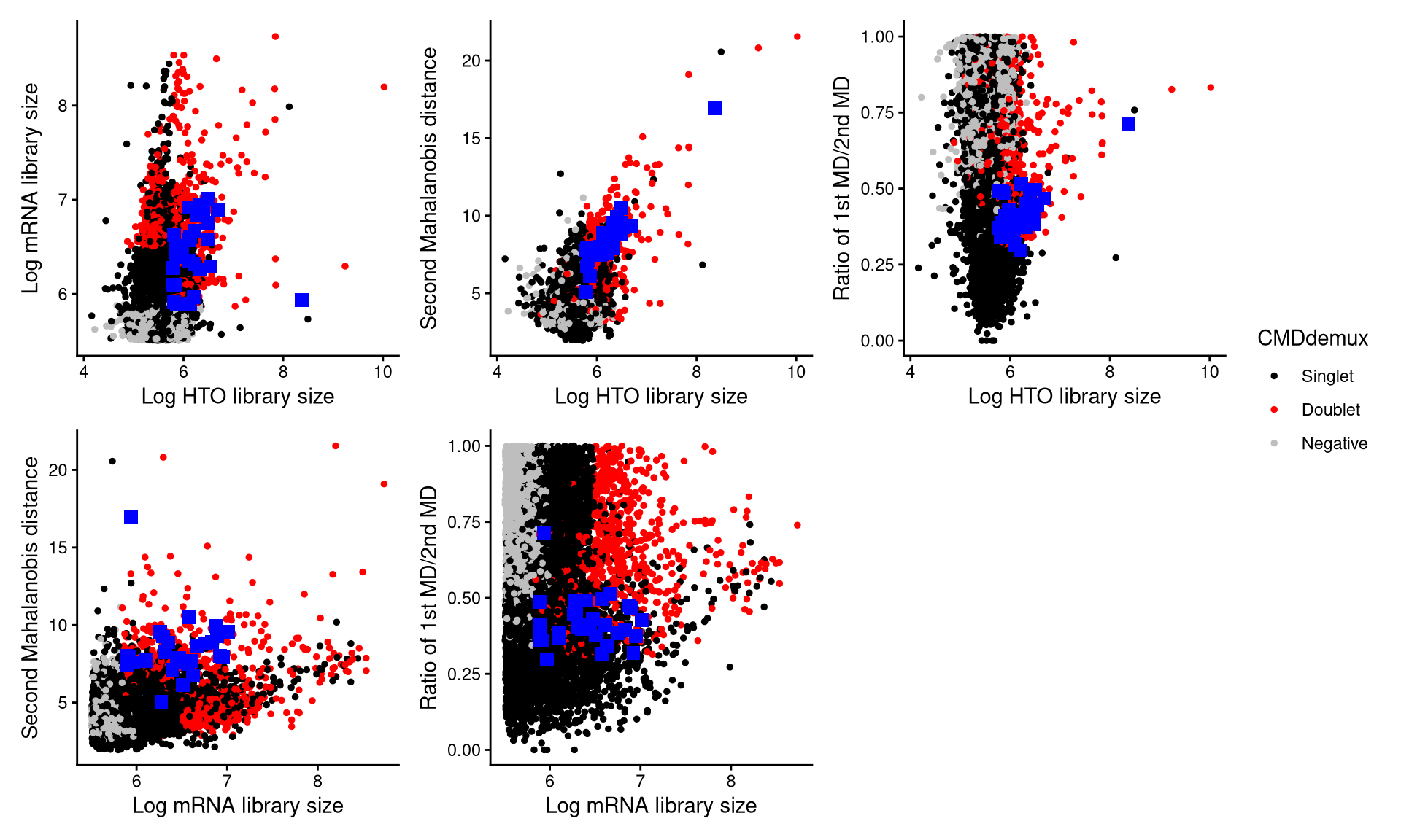
The blue squares are the randomly selected cells. Most of these cells are located in the doublet region, indicating that they should be demultiplexed as doublets.
Alternatively, we can visualize these cells using the 3D plot from CheckAssign3DPlot.
CheckAssign3DPlot(pdxhto.hash.count, pdxhto.gex.count, pdxhto.md.mat, cmddemux.assign = pdxhto.cmddemux.assign, check_barcodes = pdxhto.extra.doublet[barcode.random.idx1])The 3D plot further confirms that these cells are located in the doublet region and should be demultiplexed as doublets.
Next, we examine the cells that are demultiplexed as doublets by HTODemux but classified as HTO_3 singlets by CMDdemux. Thirty cells are randomly selected from this group.
pdxhto.extra.hto3 <- intersect(rownames(pdxhto.cmddemux.assign)[which(pdxhto.cmddemux.assign$demux_global_class == "HTO_3")], names(pdxhto.obj$HTO_classification.global)[which(pdxhto.obj$HTO_classification.global == "Doublet")])
set.seed(2026)
barcode.random.idx2 <- sample(1:length(pdxhto.extra.hto3), 30, replace = FALSE)
We then use CheckAssign2DPlot to visualize these cells in 2D.
CheckAssign2DPlot(pdxhto.hash.count, pdxhto.gex.count, pdxhto.md.mat, cmddemux.assign = pdxhto.cmddemux.assign, check_barcodes = pdxhto.extra.hto3[barcode.random.idx2], check_barcodes_col = "green", check_barcode_size = 3)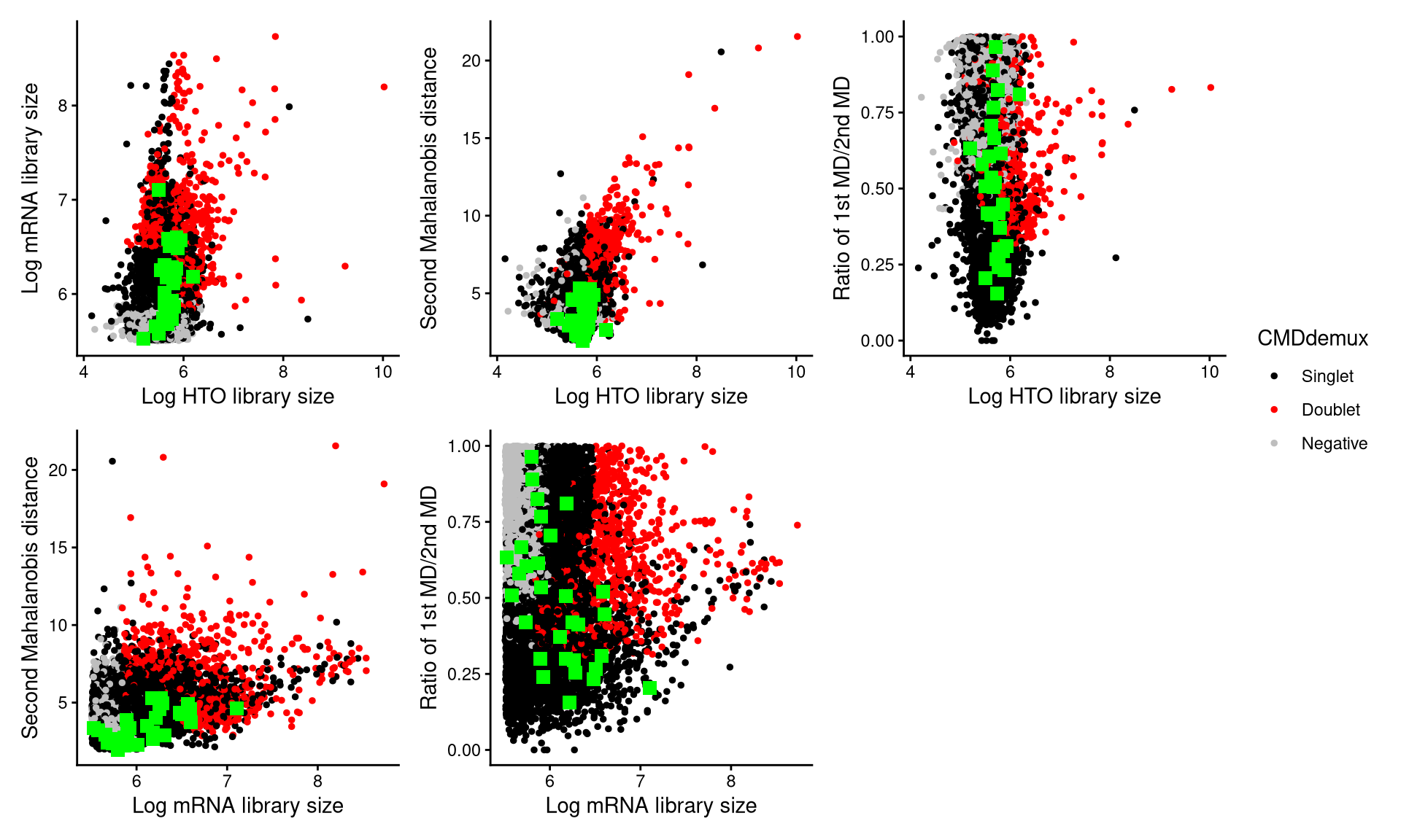
The green squares represent the randomly selected cells, and most of them are located in the singlet region, indicating that they should be demultiplexed as singlets.
We then use CheckAssign3DPlot to inspect these cells in 3D.
CheckAssign3DPlot(pdxhto.hash.count, pdxhto.gex.count, pdxhto.md.mat, cmddemux.assign = pdxhto.cmddemux.assign, check_barcodes = pdxhto.extra.hto3[barcode.random.idx2], check_barcodes_col = "green")In the 3D plot, these cells are also located in the singlet region, which further supports that they should be demultiplexed as singlets.
After that, we examine the cells that are demultiplexed as doublets by HTODemux but classified as HTO_4 singlets by CMDdemux. Thirty cells are randomly selected from this group.
pdxhto.extra.hto4 <- intersect(rownames(pdxhto.cmddemux.assign)[which(pdxhto.cmddemux.assign$demux_global_class == "HTO_4")], names(pdxhto.obj$HTO_classification.global)[which(pdxhto.obj$HTO_classification.global == "Doublet")])
set.seed(2026)
barcode.random.idx3 <- sample(1:length(pdxhto.extra.hto4), 30, replace = FALSE)
We then use CheckAssign2DPlot to visualize these cells in 2D.
CheckAssign2DPlot(pdxhto.hash.count, pdxhto.gex.count, pdxhto.md.mat, cmddemux.assign = pdxhto.cmddemux.assign, check_barcodes = pdxhto.extra.hto4[barcode.random.idx3], check_barcodes_col = "magenta", check_barcode_size = 3)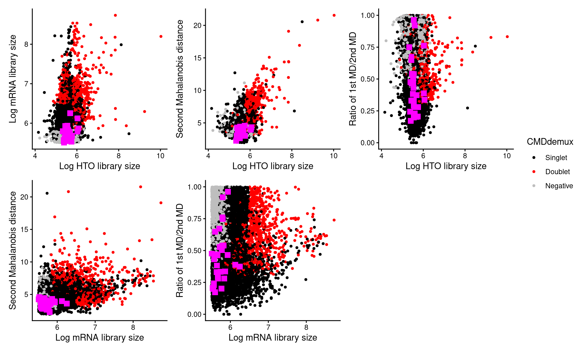
Those magenta squares represent the randomly selected cells. Most of them are located in the singlet region, so they should be demultiplexed as singlets.
We then use CheckAssign3DPlot to further confirm these cells in 3D.
CheckAssign3DPlot(pdxhto.hash.count, pdxhto.gex.count, pdxhto.md.mat, cmddemux.assign = pdxhto.cmddemux.assign, check_barcodes = pdxhto.extra.hto4[barcode.random.idx3], check_barcodes_col = "magenta")The selected cells are shown as magenta points in the plot. In the 3D plot, these cells are not located in the doublet region, which further confirms that they should not be demultiplexed as doublets, as was done by HTODemux.