Chapter 2 Human brain
This dataset is high-quality and comes from the publication (Gaublomme et al. 2019) using anti–nuclear pore complex antibodies. It includes 2,754 cells from 8 dorsolateral prefrontal cortex donors, 4 females and 4 males.
The subset of hash count data is shown below:
##       AAACCTGAGCAGGCTA-1 AAACCTGCACCAGATT-1 AAACCTGGTACTCAAC-1 AAACCTGGTATGCTTG-1 AAACCTGTCTACCAGA-1 AAACCTGTCTGGTATG-1
## S1HuF                 35                 37                 27                 46                 50                 27
## S2HuM                 26                 28                 21               3884                 89                 22
## S3HuF                 37                 32                 18                 14                 53                 21
## S4HuM                 18                 21                 30                 21                 80                 30
## S5HuF               3267                 15                  7                  8                 11                  5
## S6HuM                 15               3719                  8                 19               1146                  7
## S7HuF                 60                 53                 44                 44                 76                 49
## S8HuM                 24                 24               1709                 39                 56               1623
##       AAACGGGAGACTACAA-1 AAACGGGAGATGTAAC-1 AAACGGGAGCAATATG-1 AAACGGGCAAGAGGCT-1
## S1HuF                 52                 39                 33                 56
## S2HuM                 38                 32                 44                 36
## S3HuF                 46                 14               6684                 23
## S4HuM                 22                 22                 44                 39
## S5HuF                  7                465                  9                  7
## S6HuM                580                 12                 16                 15
## S7HuF                 47                 57                 75               1034
## S8HuM                 31                 41                 28                 54
The subset of gene expression data is shown below:
##               AAACCTGAGCAGGCTA-1 AAACCTGCACCAGATT-1 AAACCTGGTACTCAAC-1 AAACCTGGTATGCTTG-1 AAACCTGTCTACCAGA-1 AAACCTGTCTGGTATG-1
## RP11-34P13.3                   0                  0                  0                  0                  0                  0
## FAM138A                        0                  0                  0                  0                  0                  0
## OR4F5                          0                  0                  0                  0                  0                  0
## RP11-34P13.7                   0                  0                  0                  0                  0                  0
## RP11-34P13.8                   0                  0                  0                  0                  0                  0
## RP11-34P13.14                  0                  0                  0                  0                  0                  0
## RP11-34P13.9                   0                  0                  0                  0                  0                  0
## FO538757.3                     0                  0                  0                  0                  0                  0
## FO538757.2                     1                  0                  0                  0                  0                  1
## AP006222.2                     0                  0                  0                  0                  0                  0
##               AAACGGGAGACTACAA-1 AAACGGGAGATGTAAC-1 AAACGGGAGCAATATG-1 AAACGGGCAAGAGGCT-1
## RP11-34P13.3                   0                  0                  0                  0
## FAM138A                        0                  0                  0                  0
## OR4F5                          0                  0                  0                  0
## RP11-34P13.7                   0                  0                  0                  0
## RP11-34P13.8                   0                  0                  0                  0
## RP11-34P13.14                  0                  0                  0                  0
## RP11-34P13.9                   0                  0                  0                  0
## FO538757.3                     0                  0                  0                  0
## FO538757.2                     0                  0                  3                  0
## AP006222.2                     0                  0                  1                  0
2.1 Local CLR normalization
The first step of CMDdemux is to normalize the hash count data using a local CLR normalization.
##       AAACCTGAGCAGGCTA-1 AAACCTGCACCAGATT-1 AAACCTGGTACTCAAC-1 AAACCTGGTATGCTTG-1 AAACCTGTCTACCAGA-1 AAACCTGTCTGGTATG-1
## S1HuF         -0.3734377         -0.3367088         -0.2089518         0.02482044       -0.409641487        -0.18887048
## S2HuM         -0.6611197         -0.6069991         -0.4501138         4.43955110        0.158342550        -0.38558077
## S3HuF         -0.3193704         -0.4777874         -0.5967173        -1.11727696       -0.352483074        -0.43003254
## S4HuM         -1.0125176         -0.8832525         -0.1071691        -0.73428471        0.052982035        -0.08708779
## S5HuF          4.1349769         -1.2017062         -1.4617148        -1.62810259       -1.856560470        -1.72931552
## S6HuM         -1.1843679          4.2471840         -1.3439317        -0.82959489        2.703437997        -1.44163345
## S7HuF          0.1539173          0.0146891          0.2655062        -0.01866467        0.002338302         0.39094802
## S8HuM         -0.7380808         -0.7554191          3.9030923        -0.13644771       -0.298415852         3.87157253
##       AAACGGGAGACTACAA-1 AAACGGGAGATGTAAC-1 AAACGGGAGCAATATG-1 AAACGGGCAAGAGGCT-1
## S1HuF         0.17021384       -0.003142928         -0.5712813          0.2527484
## S2HuM        -0.13651643       -0.195514820         -0.2909793         -0.1793849
## S3HuF         0.05006953       -0.983972181          4.7099797         -0.6122490
## S4HuM        -0.66458386       -0.556528166         -0.2909793         -0.1014234
## S5HuF        -1.72063653        2.452163252         -1.7950567         -1.7108613
## S6HuM         2.56467268       -1.127073024         -1.2644285         -1.0177141
## S7HuF         0.07112294        0.368420629          0.2330915          3.1518539
## S8HuM        -0.33434217        0.045647237         -0.7303460          0.2170304
The output of LocalCLRNorm is a normalized data matrix with rows representing hashtag samples and columns representing cells. Each entry is a normalized value.
2.2 K-medoids clustering
Then K-medoids clustering is performed on the local CLR-normalized data.
We use a box plot to assess whether the chosen number of clusters is appropriate for the data. Each panel represents one hashtag. Ideally, in each panel, a single cluster should show much higher expression of the corresponding hashtag compared with the other clusters. This pattern indicates good clustering.
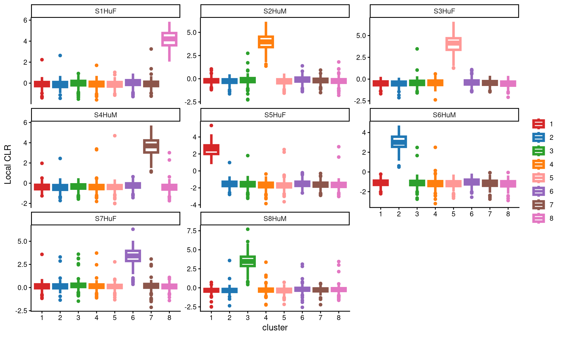
The plots above show that, in each panel, each hashtag is uniquely and highly expressed in a single cluster. This indicates clear clustering and suggests that eight clusters are sufficient for this dataset.
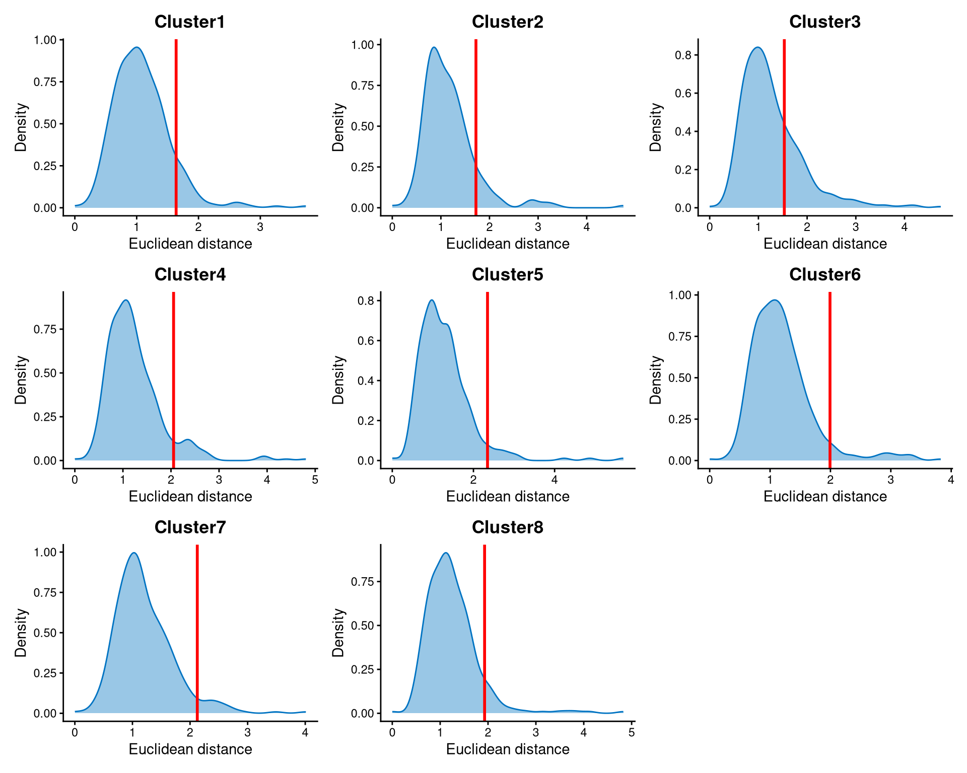
Next, we examine the distribution of the Euclidean distance of each cell to its cluster centroid within each cluster.
2.3 Definition of non-core cells
Core and non-core cells are determined by the DefineNonCore function, which requires the Euclidean distances from the output of the EuclideanClusterDist function and the clustering results from the output of the KmedCluster function. The eu_cut_q parameter can be examined using the EuclideanDistPlot function.
The basic idea for defining non-core cells is that non-core cells are those that have larger Euclidean distances and are farther away from their cluster centroids, whereas core cells are closer to their cluster centroids. A covariance matrix among clusters is required for computing the Mahalanobis distance, and we do not want non-core cells to bias this calculation. Therefore, non-core cells need to be defined in advance.
The distribution of the Euclidean distance to each cell’s cluster centroid is shown in the plot below. In the EuclideanDistPlot function, the length of the vector should match the number of clusters, and each element of the vector represents the cut-off for its corresponding cluster. The cut-off is shown as the red line, and users can adjust the parameter eu_cut_q to select different cut-offs.
hu.noncore <- DefineNonCore(hu.cl.dist, hu.kmed.cl, eu_cut_q = c(0.9, 0.9, 0.75, 0.92, 0.95, 0.94, 0.95, 0.92))
table(hu.noncore)
## hu.noncore
## Cluster1 Cluster2 Cluster3 Cluster4 Cluster5 Cluster6 Cluster7 Cluster8 non-core
## 295 215 340 338 235 384 356 306 285Next, we aim to check the definition of core and non-core cells to determine whether non-core cells are farther from the cluster centroids and core cells are closer to them.
The CLRPlot function requires the CLR-normalized values from LocalCLRNorm, the k-medoids clustering from KmedCluster, and the classified non-core cells from DefineNonCore.
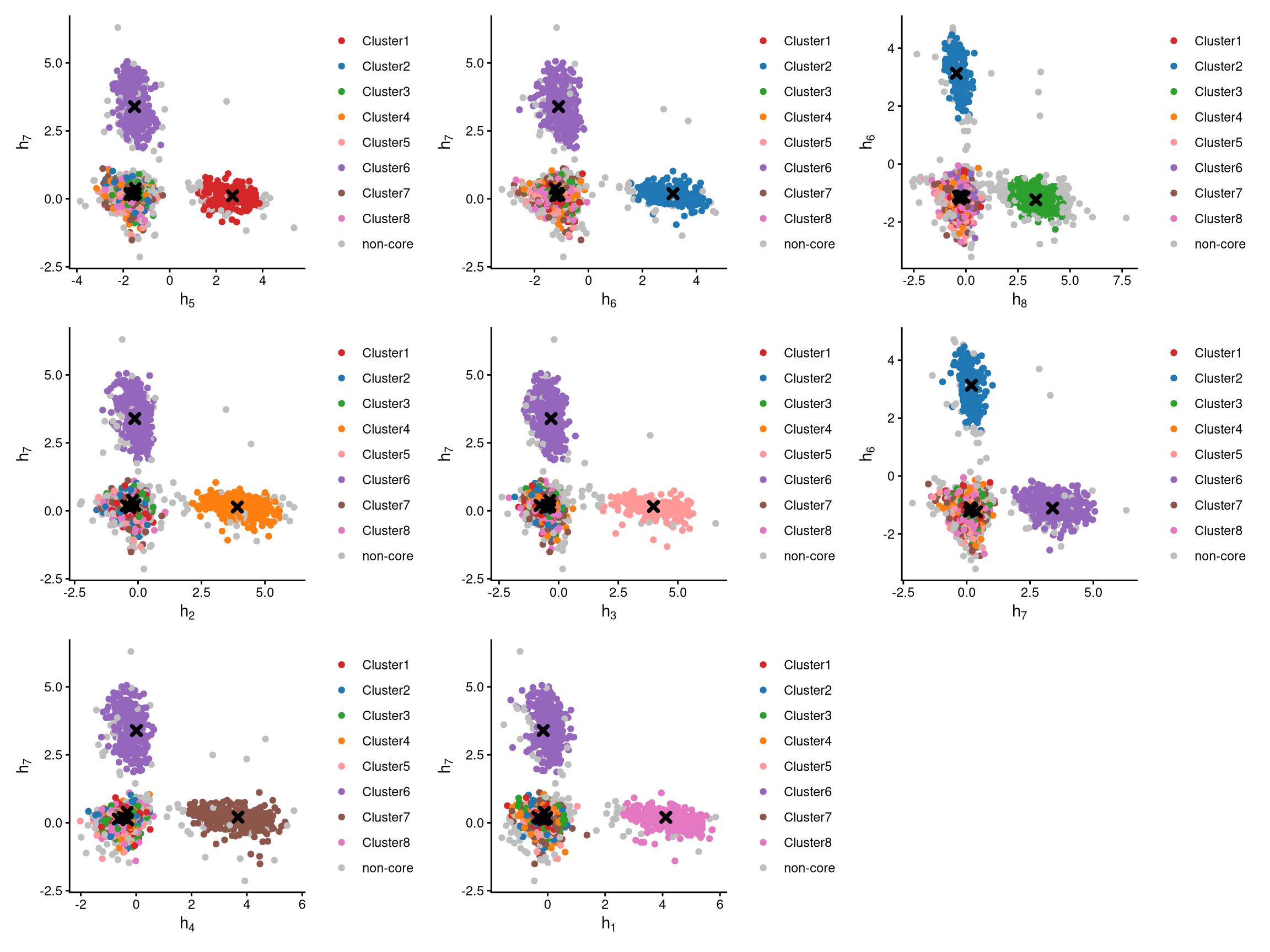
The pairwise CLR-normalized values are shown above. Each plot clearly presents two clusters of cells along with their cluster centroids. The remaining cells are positioned toward the corners. It is evident that core cells are located around the cluster centroid, whereas non-core cells are farther away from it.
2.4 Label clusters by sample
Next, we label each cluster by its original hashtag sample.
The input to LabelClusterHTO requires the CLR-normalized values from LocalCLRNorm, the k-medoids clustering from KmedCluster, and the classified non-core cells from DefineNonCore. For the label_method parameter, we commonly use the default option, but if the default does not work, we recommend using the alternative choice "expression".
hu.cluster.assign <- LabelClusterHTO(hu.clr.norm, hu.kmed.cl, hu.noncore, label_method = "medoids")
hu.cluster.assign
## S1HuF S2HuM S3HuF S4HuM S5HuF S6HuM S7HuF S8HuM
## 8 4 5 7 1 2 6 3The output above shows each sample and its corresponding cluster index.
2.5 Computing the Mahalanobis distance
The input to CalculateMD requires the CLR-normalized values from LocalCLRNorm, the k-medoids clustering from KmedCluster, the classified non-core cells from DefineNonCore, and the sample for each cluster from LabelClusterHTO.
##       AAACCTGAGCAGGCTA-1 AAACCTGCACCAGATT-1 AAACCTGGTACTCAAC-1 AAACCTGGTATGCTTG-1 AAACCTGTCTACCAGA-1 AAACCTGTCTGGTATG-1
## S1HuF          16.729513          16.734852          15.013791          14.317474           14.03400          14.948725
## S2HuM          16.264356          17.382339          15.166539           2.124494           13.49651          14.998851
## S3HuF          15.974767          15.951861          15.568014          15.512024           13.02795          15.279411
## S4HuM          16.464222          16.245151          13.677554          14.429557           12.04696          13.605766
## S5HuF           3.852669          16.421825          14.443228          14.499488           14.32579          14.757687
## S6HuM          17.021946           3.130796          15.668630          15.655158            2.37060          15.750980
## S7HuF          15.033548          16.005369          12.895535          13.425606           12.88418          12.627110
## S8HuM          16.557064          17.048728           1.747895          14.337369           13.61326           1.663073
##       AAACGGGAGACTACAA-1 AAACGGGAGATGTAAC-1 AAACGGGAGCAATATG-1 AAACGGGCAAGAGGCT-1
## S1HuF          13.040572          13.180063          16.869362          11.578491
## S2HuM          13.620153          12.942741          14.834009          12.126149
## S3HuF          12.226865          14.316151           2.128978          12.831285
## S4HuM          12.917871          12.985433          14.676813          11.580369
## S5HuF          13.978824           1.790737          15.299652          12.497210
## S6HuM           1.957518          14.301855          15.290182          13.003293
## S7HuF          12.555800          11.544650          13.810904           1.773481
## S8HuM          13.456450          12.331772          16.092512          10.418022
The output of CalculateMD is a matrix of Mahalanobis distances for each cell. Rows of the matrix correspond to hashtags, and columns correspond to cells.
2.6 Detect outlier cells
The outlier cells are defined based on the Mahalanobis distance, so it is necessary to examine the distribution of the Mahalanobis distances and determine an appropriate cut-off.
MDDensPlot is used to visualize the distribution of Mahalanobis distances. The cut-off is determined by md_cut_q, which specifies the quantile of the distribution and is shown in red. In general, we recommend selecting a cut-off near the tail of the distribution, although users can adjust this parameter.
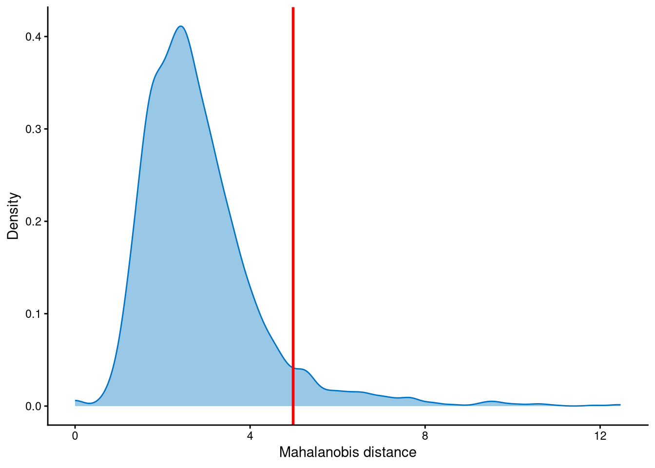
Cells with Mahalanobis distances greater than the cut-off shown in the figure are defined as outliers, whereas the remaining cells are considered singlets.
AssignOutlierDrop requires the Mahalanobis distances from CalculateMD and the md_cut_q value from the above plot to define outlier cells.
## hu.outlier.assign
## Outlier Singlet
##     166    2588
The output of AssignOutlierDrop assigns each cell as either “Outlier” or “Singlet”.”
2.7 Demultiplexing
To distinguish negatives and doublets from outlier cells, the distribution of hashtag (HTO) library sizes within outlier cells is visualized using OutlierHTOPlot.
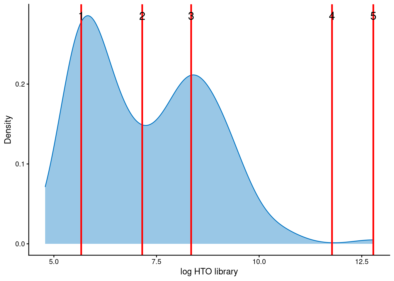
The distribution of HTO library sizes is bimodal. Cells with smaller HTO library sizes are likely negatives, whereas cells with larger HTO library sizes are likely doublets. The red lines in the plots above represent the modes and anti-modes of the distribution, which indicate potential cut-offs. The cut-off between negatives and doublets should be set at the anti-mode between the two peaks, which corresponds to index 2 of the red lines.
The final step is CMDdemux classification. Since this dataset contains gene expression data, we set use_gex_data to TRUE and provide the gene expression count data using the gex.count parameter. The num_modes parameter specifies the number of modes in the distribution, and cut_no specifies the index of the cut-off line. The appropriate number of modes and cut-off position can be determined from the OutlierHTOPlot above. For most high-quality datasets, the default values of num_modes and cut_no are sufficient.
hu.cmddemux.assign <- CMDdemuxClass(hu.md.mat, hu.hash.count, hu.outlier.assign, use_gex_data = TRUE, gex.count = hu.gex.count, num_modes = 3, cut_no = 2)
head(hu.cmddemux.assign)
## demux_id global_class demux_global_class doublet_class
## AAACCTGAGCAGGCTA-1 S5HuF Singlet S5HuF S5HuF
## AAACCTGCACCAGATT-1 S6HuM Singlet S6HuM S6HuM
## AAACCTGGTACTCAAC-1 S8HuM Singlet S8HuM S8HuM
## AAACCTGGTATGCTTG-1 S2HuM Singlet S2HuM S2HuM
## AAACCTGTCTACCAGA-1 S6HuM Singlet S6HuM S6HuM
## AAACCTGTCTGGTATG-1 S8HuM Singlet S8HuM S8HuMAn example of the output is shown above.
CMDdemux provides four types of outputs:
demux_id: the identity for each cell, determined by the sample with the minimum Mahalanobis distance for that cell.
global_class: classification of each cell as Singlet, Doublet, or Negative.
demux_global_class: singlet cells are labeled with their original sample, while negatives and doublets are labeled accordingly.
doublet_class: similar to demux_global_class, but doublets are labeled with their sample of origin. This is particularly useful for combined-hashtag experiments.
##
##  Doublet Negative    S1HuF    S2HuM    S3HuF    S4HuM    S5HuF    S6HuM    S7HuF    S8HuM
##       69       82      320      345      230      358      322      227      393      408
The output above shows the number of cells demultiplexed into each category.