Chapter 5 Treated mouse
This dataset is low-quality (Virassamy et al. 2023) and includes 4,436 cells from three mice treated with the anti-tumour drug ipatasertib. The cells were labelled using TotalSeqTM anti-mouse hashtag antibodies. The low quality of this dataset is mainly due to weak signals from the mouse 2 sample. The gene expression data is available upon request.
The subset of hash count data is shown below:
## 3 x 10 sparse Matrix of class "dgCMatrix"## [[ suppressing 10 column names 'AAACCTGAGCACAGGT', 'AAACCTGAGGACTGGT', 'AAACCTGAGTAGTGCG' ... ]]##
## mouse1 12198 30 8281 15935 23 14 31 24 18 28
## mouse2 15 8 7 6 10 . . 8 . .
## mouse3 20 17 22 42 9164 6995 9635 26 7273 9929The subset of gene expression data is shown below:
## 10 x 10 sparse Matrix of class "dgCMatrix"## [[ suppressing 10 column names 'AAACCTGAGCACAGGT', 'AAACCTGAGGACTGGT', 'AAACCTGAGTAGTGCG' ... ]]##
## Mrpl15 1 . 1 . 1 . . 1 . 2
## Lypla1 . . . . . . 1 . . 1
## Tcea1 2 . 4 2 1 1 1 . . 3
## Atp6v1h . . 2 . . . . 2 . .
## Rb1cc1 1 1 . . 1 . . . . 2
## 4732440D04Rik . . 1 . . . . . . .
## Pcmtd1 1 1 . . 3 . . . . 1
## Gm26901 . . . . . . . . . .
## Rrs1 . . . . . . . . . 1
## Mybl1 . . . . . . . . . .5.1 Local CLR normalization
The first step of CMDdemux is to normalize the hash count data using a local CLR normalization.
##        AAACCTGAGCACAGGT AAACCTGAGGACTGGT AAACCTGAGTAGTGCG AAACCTGAGTGGTAAT AAACCTGAGTTTGCGT AAACCTGCACGGTGTC AAACCTGCAGTTTACG
## mouse1         4.333702       0.59345936         4.276248         4.548521        -1.721645        -1.145664       -0.7472632
## mouse2        -2.302818      -0.64330327        -2.666150        -3.181905        -2.501803        -3.853715       -4.2129991
## mouse3        -2.030884       0.04984391        -1.610098        -1.366615         4.223448         4.999379        4.9602623
##        AAACCTGGTCTGGTCG AAACCTGGTGACTACT AAACCTGTCGCACTCT
## mouse1        0.3148967        -1.001061        -0.822908
## mouse2       -0.7067545        -3.945500        -4.190204
## mouse3        0.3918578         4.946561         5.013112
The output of LocalCLRNorm is a normalized data matrix with rows representing hashtag samples and columns representing cells. Each entry is a normalized value.
5.2 K-medoids clustering
Then K-medoids clustering is performed on the CLR-normalized data. Since there are three samples in this dataset, we use the default parameter to divide the cells into three clusters.
A boxplot is then used to check whether three clusters are appropriate for this dataset.
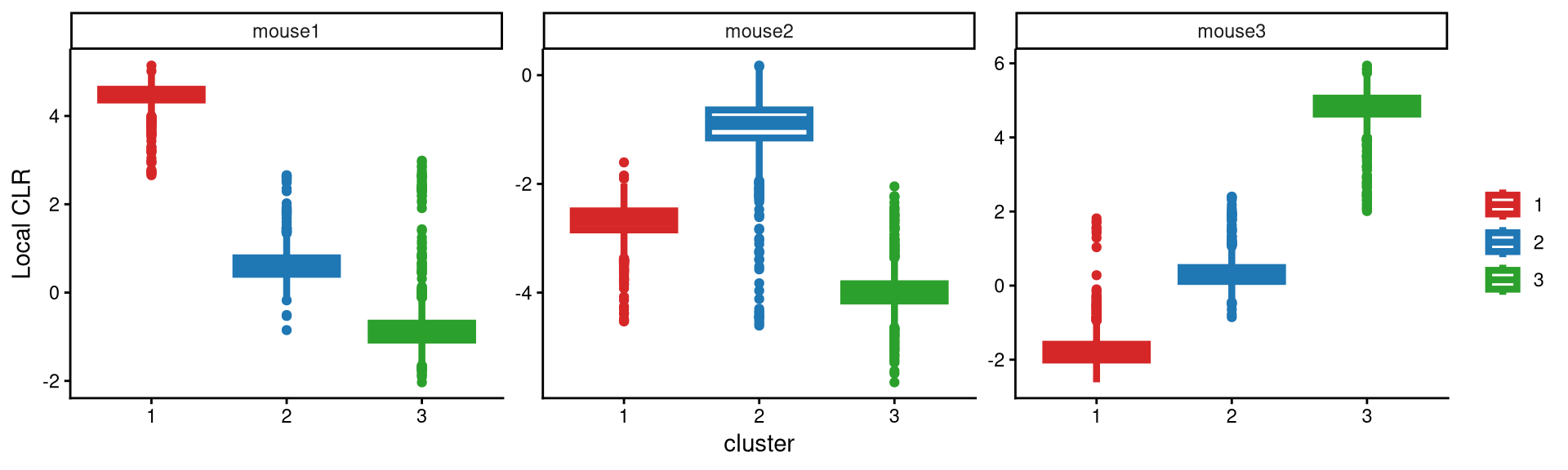
It is apparent that each hashtag sample is uniquely and highly expressed in one cluster, which indicates good clustering performance and meets our expectations. Therefore, three clusters are sufficient for this dataset.
Next, the Euclidean distance between cells and their corresponding cluster centroid within each cluster is calculated using EuclideanClusterDist.
5.3 Definition of non-core cells
Core cells are defined as cells that are closer to their cluster centroids, while non-core cells are those that are farther away from the cluster centroid. The cut-off between core and non-core cells can be determined using EuclideanDistPlot, which visualizes the cut-off based on the quantile of the distribution via the eu_cut_q parameter, shown as the red line in the plot.
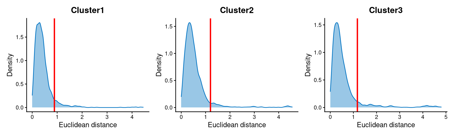
The distribution of Euclidean distances within each cluster is right-skewed. The cut-offs are set at the tail of each distribution, so cells with Euclidean distances beyond the cut-off are defined as non-core cells, while the others are defined as core cells.
Core and non-core cells are then classified using DefineNonCore, applying the eu_cut_q parameter selected from the above plot.
treated.noncore <- DefineNonCore(treated.cl.dist, treated.kmed.cl, eu_cut_q = c(0.93, 0.94, 0.91))
table(treated.noncore)
## treated.noncore
## Cluster1 Cluster2 Cluster3 non-core
## 1539 1260 1310 327Core cells are labelled by their clusters, and non-core cells are directly labelled as “non-core.”
The definition of core and non-core cells is further examined using CLRPlot.
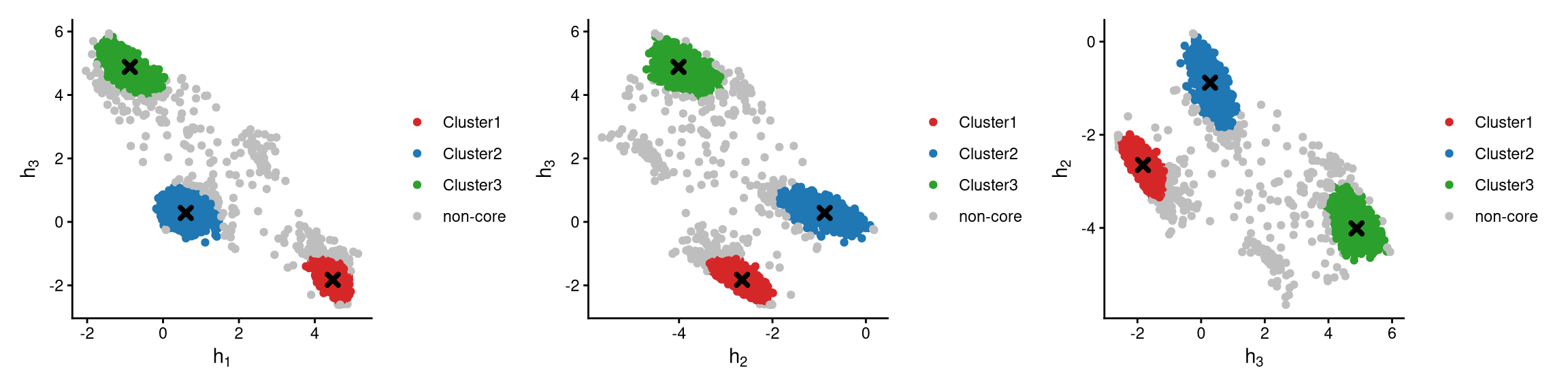
The pairwise CLR-normalized values are shown in the above plots. Cells are grouped by clusters, and cluster centroids are indicated by cross symbols. It is apparent that non-core cells are further away from the cluster centroids, while core cells are located around the centroids.
5.4 Label clusters by sample
Each cluster will be labelled with its original sample, and here we use the default medoid-based labelling method.
treated.cluster.assign <- LabelClusterHTO(treated.clr.norm, treated.kmed.cl, treated.noncore, label_method = "medoids")
treated.cluster.assign
## mouse1 mouse2 mouse3
## 1 2 3The results show each sample and its corresponding cluster index. For example, cluster 1 corresponds to the mouse1 sample.
5.5 Computing the Mahalanobis distance
Using the local CLR-normalized values from LocalCLRNorm, the non-core cell classifications from DefineNonCore, the k-medoids clustering from KmedCluster, and the cluster labelling from LabelClusterHTO, the Mahalanobis distance for each single cell can be calculated using CalculateMD.
treated.md.mat <- CalculateMD(treated.clr.norm, treated.noncore, treated.kmed.cl, treated.cluster.assign)
treated.md.mat[,1:10]
## AAACCTGAGCACAGGT AAACCTGAGGACTGGT AAACCTGAGTAGTGCG AAACCTGAGTGGTAAT AAACCTGAGTTTGCGT AAACCTGCACGGTGTC AAACCTGCAGTTTACG
## mouse1 1.252352 16.2713600 0.9607986 2.021603 28.727790 28.780931 27.8101896
## mouse2 15.782087 0.9484528 15.4181923 16.589489 14.957720 17.247954 17.1955351
## mouse3 28.105135 17.7336692 26.9412402 27.015989 5.598405 1.140203 0.7704736
## AAACCTGGTCTGGTCG AAACCTGGTGACTACT AAACCTGTCGCACTCT
## mouse1 17.457287 28.3278948 28.1002961
## mouse2 1.200757 17.0641998 17.3633320
## mouse3 16.565672 0.5320873 0.6583967The output is a Mahalanobis distance matrix with rows representing hashtag samples and columns representing cells. Each entry indicates the Mahalanobis distance of a cell to a given hashtag sample.
5.6 Detect outlier cells
Outlier cells, including negatives and doublets, are defined based on the distribution of the minimum Mahalanobis distance across all cells, which can be visualized using MDDensPlot. The cut-off in the plot is determined by the md_cut_q parameter, which specifies the quantile of the distribution and is shown as the red line. Users are encouraged to adjust the cut-off through the md_cut_q parameter.
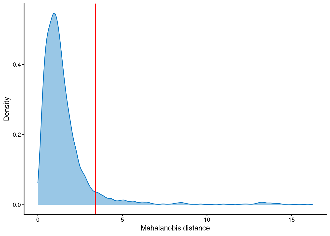
The distribution of Mahalanobis distances is right-skewed, and we set the cut-off at the tail of the distribution. Cells with Mahalanobis distances larger than this cut-off are defined as outlier cells, as they are considered to be further away from the cluster centroids, while the others are defined as core cells, which are closer to the centroids.
Outlier cells are then defined using AssignOutlierDrop according to the cut-off selected from the plot.
treated.outlier.assign <- AssignOutlierDrop(treated.md.mat, md_cut_q = 0.93)
table(treated.outlier.assign )
## treated.outlier.assign
## Outlier Singlet
## 311 4125In this step, cells are labelled as either outliers or singlets.
5.7 Demultiplexing
The HTO library sizes are used to further distinguish negatives and doublets among the outlier cells. The distribution of HTO library sizes can be visualized using OutlierHTOPlot. The possible cut-offs corresponding to the modes and anti-modes are shown as red lines in the plot.
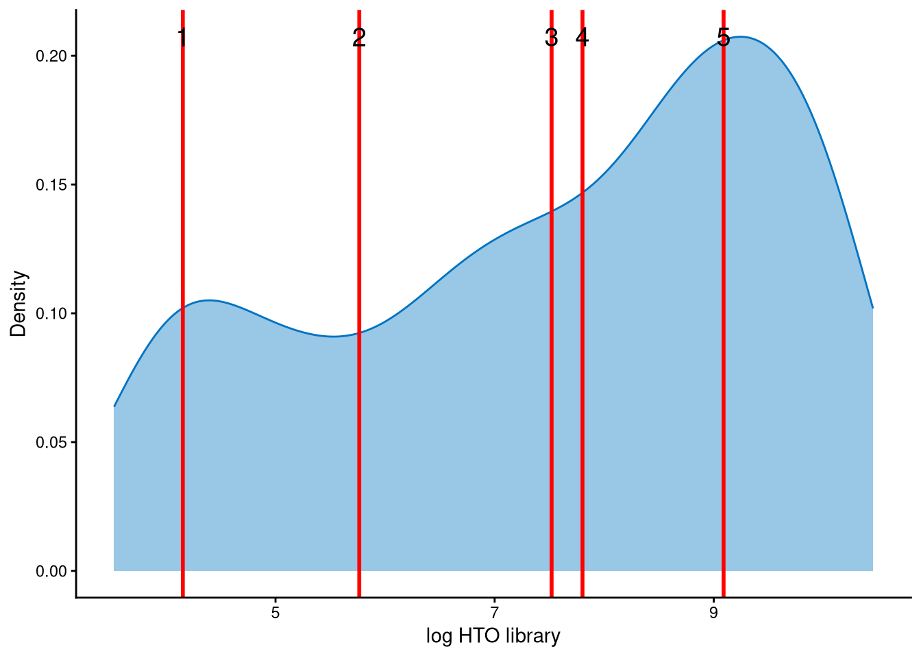
This dataset is approximately bimodally distributed. The peak with smaller HTO library sizes corresponds to negatives, while the peak with larger HTO library sizes corresponds to doublets. Therefore, line index 2 is an appropriate cut-off to distinguish negatives from doublets.
treated.cmddemux.assign <- CMDdemuxClass(treated.md.mat, treated.hash.count, treated.outlier.assign, use_gex_data = TRUE, gex.count = treated.gex.count, cut_no = 2)
head(treated.cmddemux.assign)
## demux_id global_class demux_global_class doublet_class
## AAACCTGAGCACAGGT mouse1 Singlet mouse1 mouse1
## AAACCTGAGGACTGGT mouse2 Singlet mouse2 mouse2
## AAACCTGAGTAGTGCG mouse1 Singlet mouse1 mouse1
## AAACCTGAGTGGTAAT mouse1 Singlet mouse1 mouse1
## AAACCTGAGTTTGCGT mouse3 Doublet Doublet mouse2_mouse3
## AAACCTGCACGGTGTC mouse3 Singlet mouse3 mouse3The gene expression data also helps with demultiplexing, and the cut-off selected from the above plot is applied here as well.
CMDdemux provides four types of outputs:
demux_id: the identity for each cell, determined by the sample with the minimum Mahalanobis distance for that cell.
global_class: classification of each cell as Singlet, Doublet, or Negative.
demux_global_class: singlet cells are labeled with their original sample, while negatives and doublets are labeled accordingly.
doublet_class: similar to demux_global_class, but doublets are labeled with their sample of origin. This is particularly useful for combined-hashtag experiments.
##
##  Doublet   mouse1   mouse2   mouse3 Negative
##      115     1637     1275     1353       56
The output above shows the number of cells demultiplexed into each category.