Chapter 11 PDX MULTI-Seq CMO
This dataset is low quality (Brown et al. 2024) and contains 4,178 cells derived from a human ovarian carcinosarcoma patient-derived xenograft (PDX). Nuclei from four donors were labelled using custom MULTI-Seq cholesterol-modified oligos (CMOs). The low quality is due to the low input, with all hashtag labels showing weak signals. In addition, the dataset suffers from uneven labelling, with Nxt_451 and Nxt_452 exhibiting much stronger signals compared with the other hashtags.
The subset of hash count data is shown below:
## 4 x 10 sparse Matrix of class "dgCMatrix"## [[ suppressing 10 column names 'AAACCCACAGCCCAGT-1', 'AAACCCAGTATGCGGA-1', 'AAACCCAGTCATCGGC-1' ... ]]##
## Nxt_451 325 143 405 157 436 136 132 149 161 330
## Nxt_452 398 969 346 780 576 313 913 326 183 664
## Nxt_453 152 29 24 20 28 244 24 146 8 17
## Nxt_455 25 40 43 44 45 21 29 39 18 25The subset of gene expression data is shown below:
## 10 x 10 sparse Matrix of class "dgCMatrix"## [[ suppressing 10 column names 'AAACCCACAGCCCAGT-1', 'AAACCCAGTATGCGGA-1', 'AAACCCAGTCATCGGC-1' ... ]]##
## AL627309.1 . . . . . . . . . .
## AL627309.2 . . . . . . . . . .
## AL627309.5 . . . . . . . . . .
## AL627309.4 . . . . . . . . . .
## AL669831.2 . . . . . . . . . .
## LINC01409 . . . . . . . . . .
## FAM87B . . . . . . . . . .
## LINC01128 . . . . . . . . . .
## LINC00115 . . . . . . . . . .
## FAM41C . . . . . . . . . .11.1 Local CLR normalization
The first step of CMDdemux is to normalize the hash count data using a local CLR normalization.
##         AAACCCACAGCCCAGT-1 AAACCCAGTATGCGGA-1 AAACCCAGTCATCGGC-1 AAACCCATCACCTACC-1 AAACCCATCACTTGGA-1 AAACGAAAGTTGTAAG-1
## Nxt_451         0.77079907          0.2293436          1.2916673          0.4190063           1.171505          0.1045623
## Nxt_452         0.97286310          2.1368264          1.1346389          2.0169864           1.449414          0.9339743
## Nxt_453         0.01433961         -1.3392723         -1.4958100         -1.5990663          -1.541132          0.6858396
## Nxt_455        -1.75800178         -1.0268976         -0.9304962         -0.8369263          -1.079787         -1.7243762
##         AAACGAATCCCATACC-1 AAACGAATCGGTCTGG-1 AAACGCTAGGGTTAGC-1 AAACGCTCAGCTCGGT-1
## Nxt_451          0.3082859          0.1406584          1.2265474           1.189525
## Nxt_452          2.2357673          0.9199833          1.3538868           1.887194
## Nxt_453         -1.3631874          0.1204557         -1.6638243          -1.722222
## Nxt_455         -1.1808658         -1.1810974         -0.9166099          -1.354497
The output of LocalCLRNorm is a normalized data matrix with rows representing hashtag samples and columns representing cells. Each entry is a normalized value.
11.2 K-medoids clustering
The local CLR-normalized values are used here for K-medoids clustering. Since this dataset has four samples, the default parameters are applied, which divides the cells into four clusters.
A boxplot is then used to check whether four clusters are appropriate for this dataset.
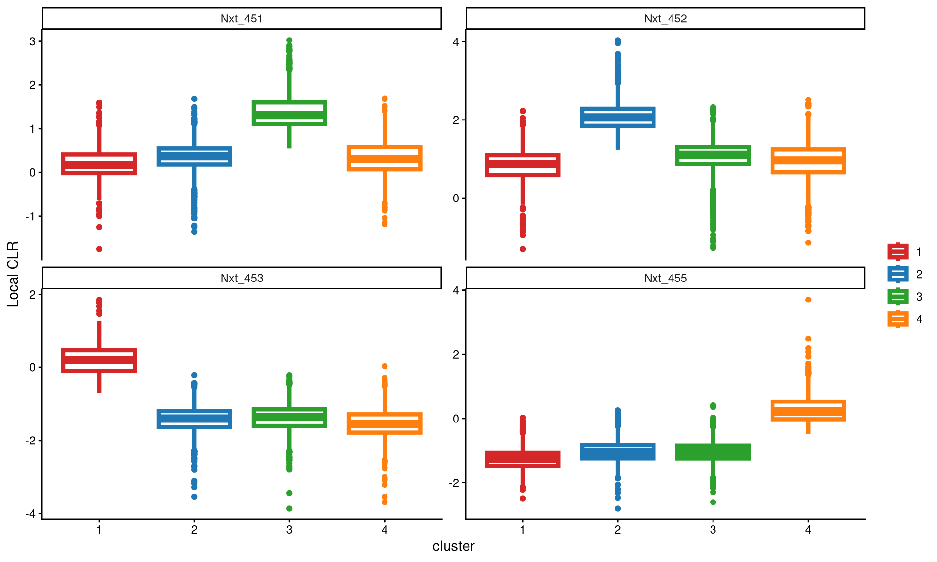
The box plot shows that each hashtag sample is highly and uniquely expressed in one cluster, indicating that four clusters are ideal for this dataset.
Next, the Euclidean distance between cells and their corresponding cluster centroid within each cluster is calculated using EuclideanClusterDist.
11.3 Definition of non-core cells
Core cells are defined as cells that are closer to their cluster centroids, while non-core cells are those that are farther away from the cluster centroid. The cut-off between core and non-core cells can be determined using EuclideanDistPlot, which visualizes the cut-off based on the quantile of the distribution via the eu_cut_q parameter, shown as the red line in the plot. Each value in the eu_cut_q parameter corresponds to a cut-off for a cluster.
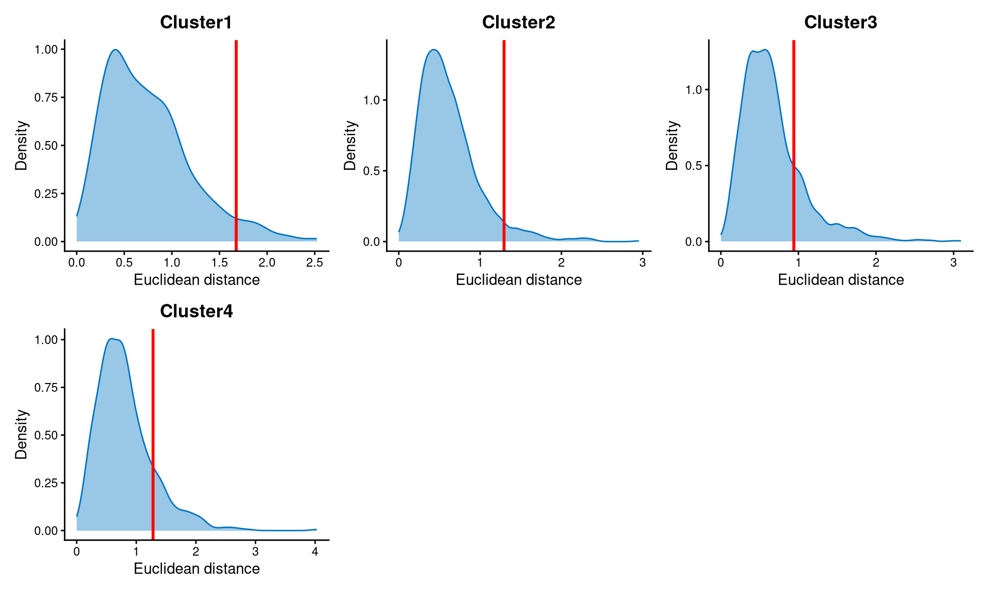
The Euclidean distance for each of the four clusters follows a right-skewed distribution, and the cut-off is defined at the tail of the distribution.
Core and non-core cells are then classified using DefineNonCore, applying the eu_cut_q parameter selected from the above plot.
pdxnxt.noncore <- DefineNonCore(pdxnxt.cl.dist, pdxnxt.kmed.cl, eu_cut_q = c(0.95, 0.95, 0.81, 0.86))
table(pdxnxt.noncore)
## pdxnxt.noncore
## Cluster1 Cluster2 Cluster3 Cluster4 non-core
## 461 1361 1224 642 490Core cells are labelled by their clusters, and non-core cells are directly labelled as “non-core.”
The definition of core and non-core cells is further examined using CLRPlot.
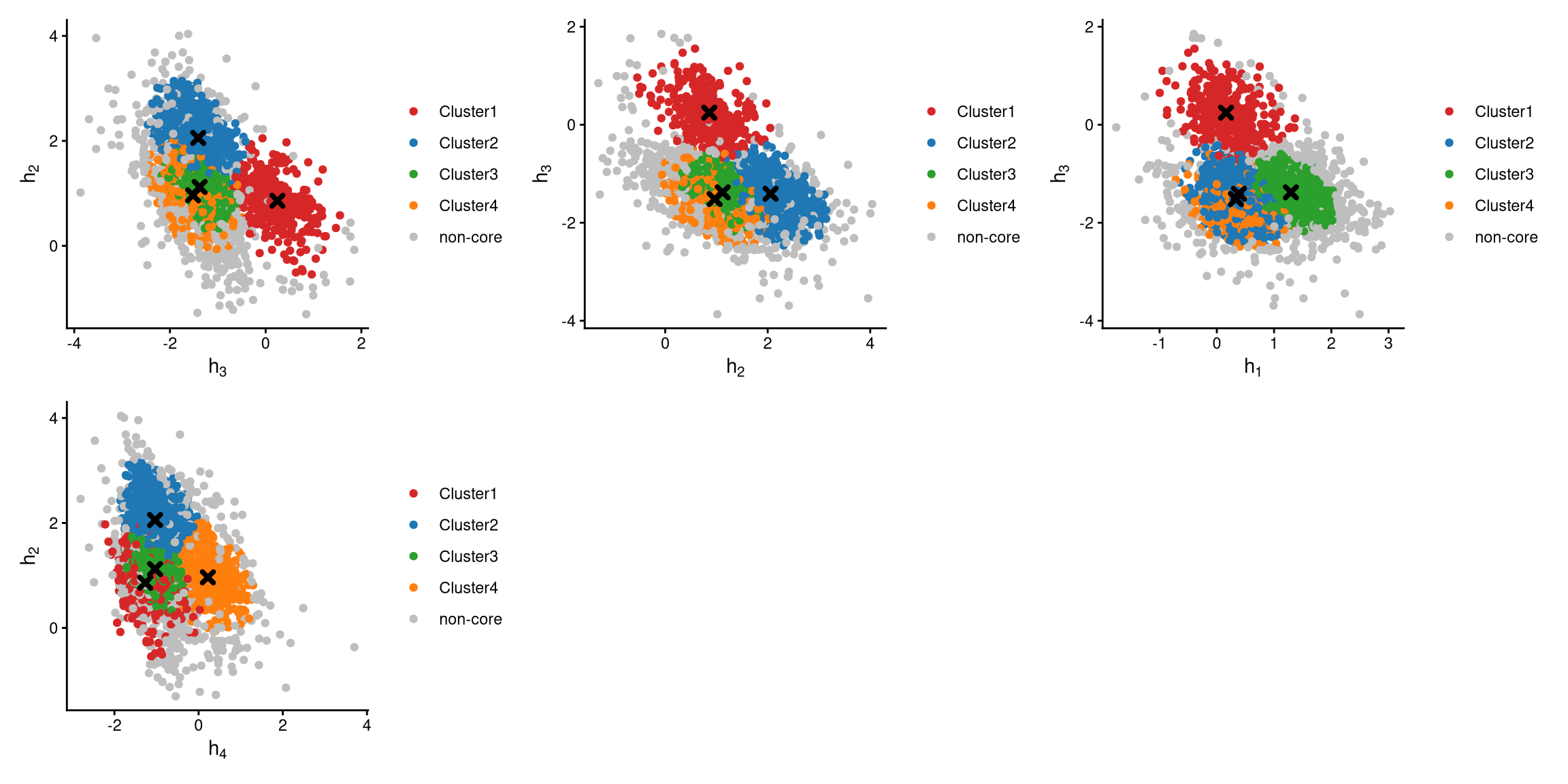
The pairwise local CLR-normalized values are shown in the above plots. Each plot clearly demonstrates two clusters, with other clusters appearing in the corners. Cluster centroids are indicated by cross symbols. Core cells cluster around the centroids, whereas non-core cells lie at the edges of the clusters.
11.4 Label clusters by sample
Each cluster will be labelled with its original sample, and here we use the default medoid-based labelling method.
pdxnxt.cluster.assign <- LabelClusterHTO(pdxnxt.clr.norm, pdxnxt.kmed.cl, pdxnxt.noncore, label_method = "medoids")
pdxnxt.cluster.assign
## Nxt_451 Nxt_452 Nxt_453 Nxt_455
## 3 2 1 4The results show each sample and its corresponding cluster index. For example, cluster 1 corresponds to the Nxt_453 sample.
11.5 Computing the Mahalanobis distance
Using the local CLR-normalized values from LocalCLRNorm, the non-core cell classifications from DefineNonCore, the k-medoids clustering from KmedCluster, and the cluster labelling from LabelClusterHTO, the Mahalanobis distance for each single cell can be calculated using CalculateMD.
pdxnxt.md.mat <- CalculateMD(pdxnxt.clr.norm, pdxnxt.noncore, pdxnxt.kmed.cl, pdxnxt.cluster.assign)
pdxnxt.md.mat[,1:10]
## AAACCCACAGCCCAGT-1 AAACCCAGTATGCGGA-1 AAACCCAGTCATCGGC-1 AAACCCATCACCTACC-1 AAACCCATCACTTGGA-1 AAACGAAAGTTGTAAG-1
## Nxt_451 4.571640 3.9441973 0.4314271 3.3746116 0.9861782 6.854932
## Nxt_452 5.060933 0.5265755 3.4980161 0.7856426 2.7206466 6.504643
## Nxt_453 2.280370 5.2301447 5.8110638 5.7827395 5.7738674 1.802286
## Nxt_455 7.064090 4.7948739 4.1964374 4.1080166 4.5268372 8.186933
## AAACGAATCCCATACC-1 AAACGAATCGGTCTGG-1 AAACGCTAGGGTTAGC-1 AAACGCTCAGCTCGGT-1
## Nxt_451 3.9968756 5.2437809 0.9995259 2.335712
## Nxt_452 0.6897187 4.9455127 3.1008313 2.588509
## Nxt_453 5.4115155 0.4375366 6.1504789 6.482349
## Nxt_455 5.2772101 6.0046942 4.1866173 5.624634The output is a Mahalanobis distance matrix with rows representing hashtag samples and columns representing cells. Each entry indicates the Mahalanobis distance of a cell to a given hashtag sample.
11.6 Detect outlier cells
Outlier cells, including negatives and doublets, are defined based on the distribution of the minimum Mahalanobis distance across all cells, which can be visualized using MDDensPlot. The cut-off in the plot is determined by the md_cut_q parameter, which specifies the quantile of the distribution and is shown as the red line. Users are encouraged to adjust the cut-off through the md_cut_q parameter.
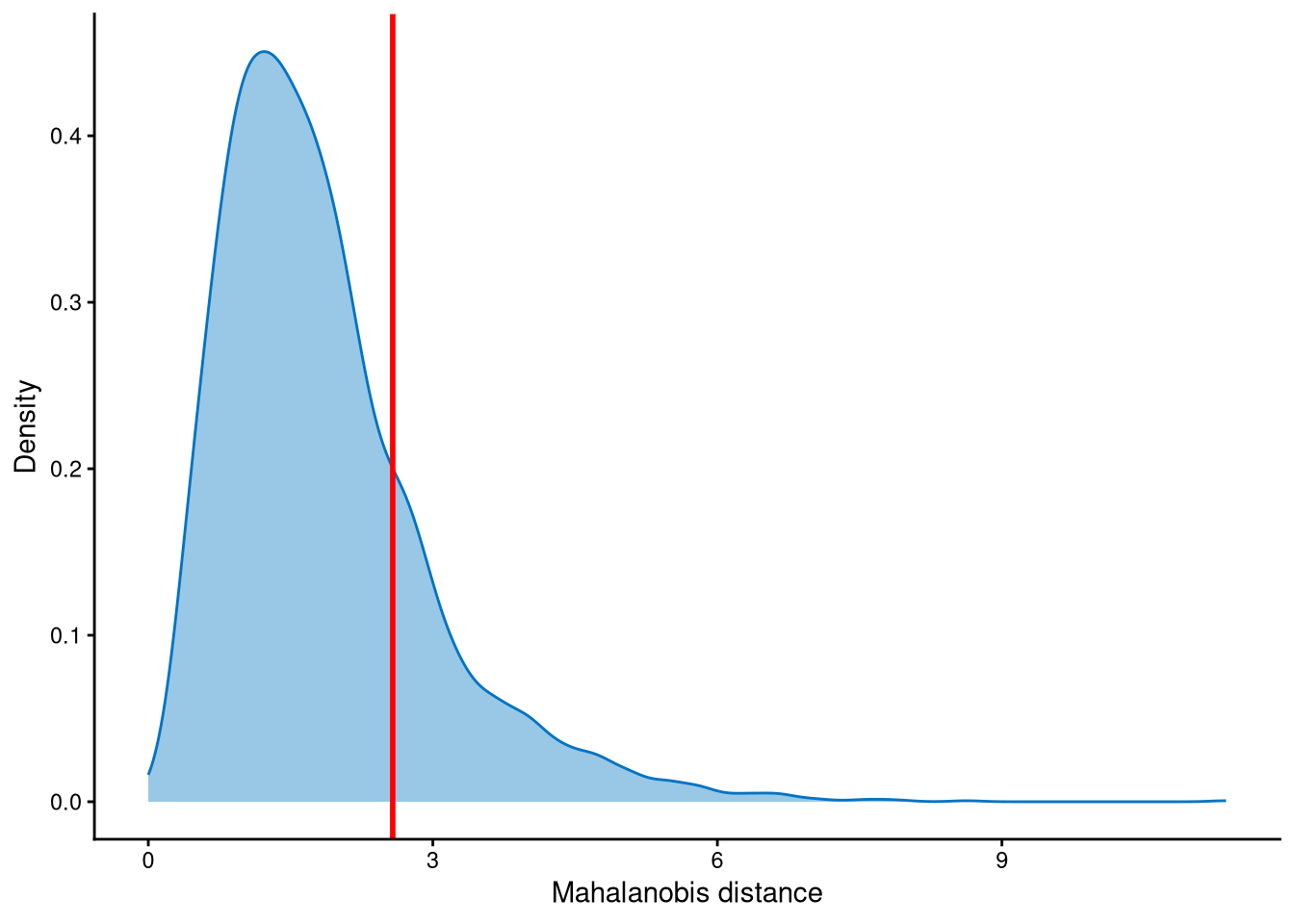
The distribution of Mahalanobis distances is right-skewed, and the cut-off is set at the tail of the distribution.
Outlier cells are then defined using AssignOutlierDrop according to the cut-off selected from the plot.
pdxnxt.outlier.assign <- AssignOutlierDrop(pdxnxt.md.mat, md_cut_q = 0.8)
table(pdxnxt.outlier.assign)
## pdxnxt.outlier.assign
## Outlier Singlet
## 836 3342In this step, cells are labelled as either outliers or singlets.
11.7 Demultiplexing
The HTO library sizes are used to further distinguish negatives and doublets among the outlier cells. The distribution of HTO library sizes can be visualized using OutlierHTOPlot. The possible cut-offs corresponding to the modes and anti-modes are shown as red lines in the plot. The parameter num_modes is used to set the number of modes in the plot.
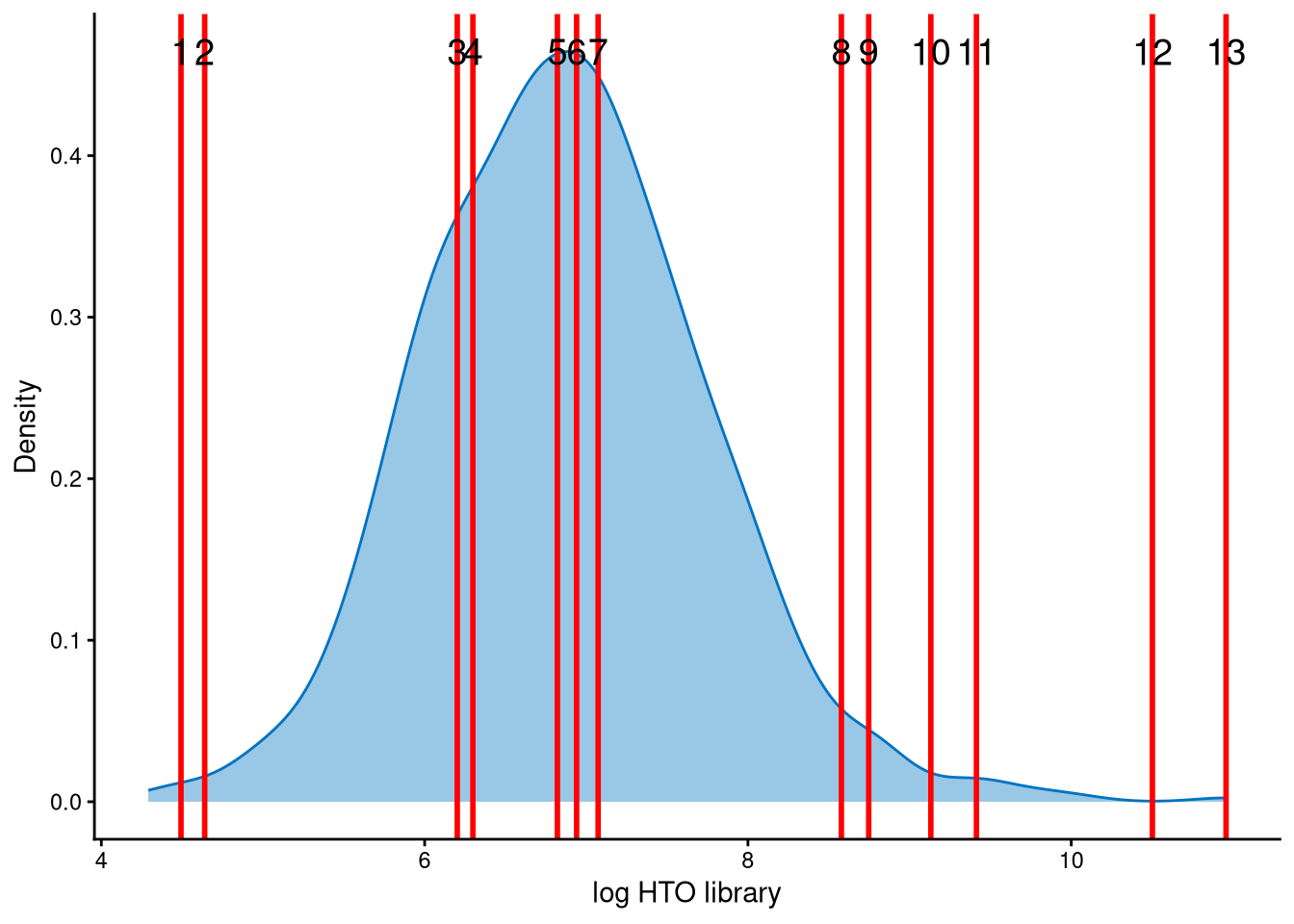
The distribution of HTO library sizes is not a typical bimodal distribution; therefore, the cut-off should be set at a reasonable value. For lines 1 and 2, the HTO library size (total hashtag counts per cell) is approximately \(e^4\approx55\), which is too small. In contrast, for lines 3 and 4, the HTO library size is approximately \(e^{6.2}\approx493\), which is more reasonable than that of lines 1 and 2. Therefore, the final cut-off is set at line 4.
In the final step of demultiplexing, the Mahalanobis distance from CalculateMD, the original hashtag count matrix, the outlier classifications from AssignOutlierDrop, the gene expression data, and the selected HTO library size cut-off from the above plot are applied.
pdxnxt.cmddemux.assign <- CMDdemuxClass(pdxnxt.md.mat, pdxnxt.hash.count, pdxnxt.outlier.assign, use_gex_data = TRUE, gex.count = pdxnxt.gex.count, num_modes = 7, cut_no = 4)
head(pdxnxt.cmddemux.assign)
## demux_id global_class demux_global_class doublet_class
## AAACCCACAGCCCAGT-1 Nxt_453 Singlet Nxt_453 Nxt_453
## AAACCCAGTATGCGGA-1 Nxt_452 Singlet Nxt_452 Nxt_452
## AAACCCAGTCATCGGC-1 Nxt_451 Singlet Nxt_451 Nxt_451
## AAACCCATCACCTACC-1 Nxt_452 Singlet Nxt_452 Nxt_452
## AAACCCATCACTTGGA-1 Nxt_451 Singlet Nxt_451 Nxt_451
## AAACGAAAGTTGTAAG-1 Nxt_453 Singlet Nxt_453 Nxt_453CMDdemux provides four types of outputs:
demux_id: the identity for each cell, determined by the sample with the minimum Mahalanobis distance for that cell.
global_class: classification of each cell as Singlet, Doublet, or Negative.
demux_global_class: singlet cells are labeled with their original sample, while negatives and doublets are labeled accordingly.
doublet_class: similar to demux_global_class, but doublets are labeled with their sample of origin. This is particularly useful for combined-hashtag experiments.
##
##  Doublet Negative  Nxt_451  Nxt_452  Nxt_453  Nxt_455
##      511      118     1295     1287      391      576
The output above shows the number of cells demultiplexed into each category.
11.8 Examination of suspicious droplets
In the original paper, CMDdemux demultiplexes more singlets in Nxt_451 and Nxt_452, whereas HTODemux demultiplexes them as negatives. We can use the functions CheckAssign2DPlot and CheckAssign3DPlot to visually assess whether the CMDdemux assignments are correct.
CheckAssign2DPlot consists of pairwise 2D plots of HTO library sizes, mRNA library sizes, the second Mahalanobis distance, and the ratio of the first to the second Mahalanobis distance. Negatives, singlets, and doublets are separated into different regions in these 2D plots.
CheckAssign3DPlot uses HTO library sizes, mRNA library sizes, and the ratio of the first to the second Mahalanobis distance to visualize negatives, singlets, and doublets in 3D.
First, apply HTODemux to the data.
pdxnxt.obj <- CreateSeuratObject(counts = pdxnxt.hash.count)
pdxnxt.obj[["HTO"]] <- CreateAssayObject(counts = pdxnxt.hash.count)
pdxnxt.obj <- NormalizeData(pdxnxt.obj, assay = "HTO", normalization.method = "CLR")
pdxnxt.obj <- HTODemux(pdxnxt.obj, assay = "HTO", positive.quantile = 0.99)
We then examine the cells that are assigned as Nxt_451 singlets by CMDdemux but classified as negatives by HTODemux. For this examination, 30 cells are randomly selected from this group.
pdxnxt.extra.nxt451 <- intersect(rownames(pdxnxt.cmddemux.assign)[which(pdxnxt.cmddemux.assign$demux_global_class == "Nxt_451")], names(pdxnxt.obj$HTO_classification.global)[which(pdxnxt.obj$HTO_classification.global == "Negative")])
set.seed(2026)
barcode.random.idx1 <- sample(1:length(pdxnxt.extra.nxt451), 30, replace = FALSE)
We then use CheckAssign2DPlot to visualize these cells in 2D.
CheckAssign2DPlot(pdxnxt.hash.count, pdxnxt.gex.count, pdxnxt.md.mat, cmddemux.assign = pdxnxt.cmddemux.assign, check_barcodes = pdxnxt.extra.nxt451[barcode.random.idx1], check_barcode_size = 3)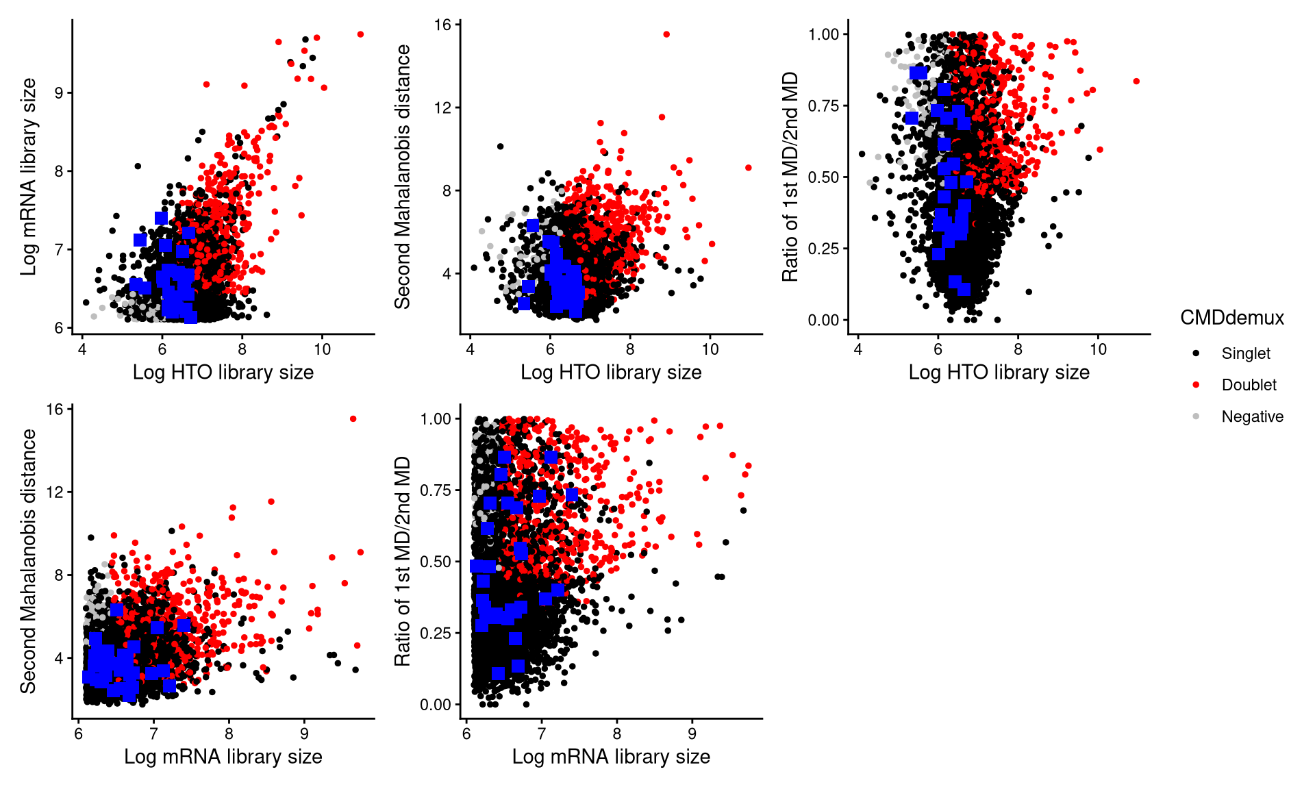
The blue squares in the plot represent the randomly selected cells. Most of them are located in the singlet region, indicating that they should be demultiplexed as singlets.
We then use CheckAssign3DPlot to inspect these cells in 3D.
CheckAssign3DPlot(pdxnxt.hash.count, pdxnxt.gex.count, pdxnxt.md.mat, cmddemux.assign = pdxnxt.cmddemux.assign, check_barcodes = pdxnxt.extra.nxt451[barcode.random.idx1])The blue dots in the 3D plot are the randomly selected cells. Most of them are located in the singlet region, which further supports that they are correctly demultiplexed as singlets by CMDdemux.
Next, we examine the cells that are demultiplexed as Nxt_452 singlets by CMDdemux but as negatives by HTODemux. Thirty cells are randomly selected from this group.
pdxnxt.extra.nxt452 <- intersect(rownames(pdxnxt.cmddemux.assign)[which(pdxnxt.cmddemux.assign$demux_global_class == "Nxt_452")], names(pdxnxt.obj$HTO_classification.global)[which(pdxnxt.obj$HTO_classification.global == "Negative")])
set.seed(2026)
barcode.random.idx2 <- sample(1:length(pdxnxt.extra.nxt452), 30, replace = FALSE)
We then use CheckAssign2DPlot to visualize these cells in 2D.
CheckAssign2DPlot(pdxnxt.hash.count, pdxnxt.gex.count, pdxnxt.md.mat, cmddemux.assign = pdxnxt.cmddemux.assign, check_barcodes = pdxnxt.extra.nxt452[barcode.random.idx2], check_barcodes_col = "green", check_barcode_size = 3)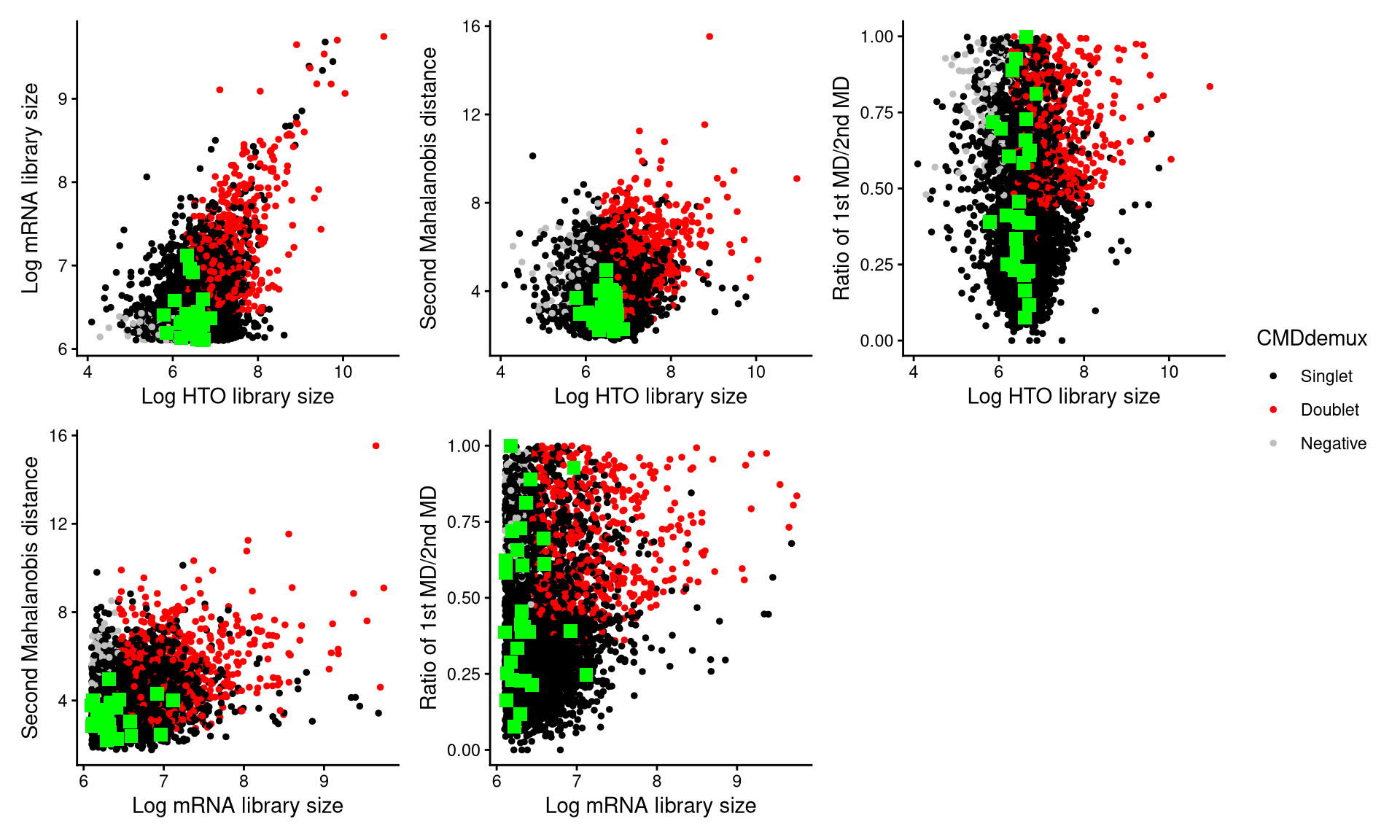
Those randomly selected cells are shown as green squares in the plot. Most of them are located in the singlet region, suggesting that they should be demultiplexed as singlets.
We then use CheckAssign3DPlot to inspect these cells in 3D.
CheckAssign3DPlot(pdxnxt.hash.count, pdxnxt.gex.count, pdxnxt.md.mat, cmddemux.assign = pdxnxt.cmddemux.assign, check_barcodes = pdxnxt.extra.nxt452[barcode.random.idx2], check_barcodes_col = "green")The randomly selected cells are shown as green dots in the 3D plot. Most of them are in the singlet area, which further supports that CMDdemux correctly demultiplexes them as Nxt_452 singlets.