Chapter 12 PBMC
This dataset (Stoeckius et al. 2018) includes 21,522 peripheral blood mononuclear cells (PBMCs) from eight human donors, which were labelled with antibody oligos. The quality of this dataset is high, and many methods use it as an example dataset to demonstrate their approaches. However, it contains many more empty droplets than other datasets, which poses challenges for clustering. Therefore, I include it here as a low-quality example.
The subset of hash count data is shown below:
## 8 x 10 sparse Matrix of class "dgCMatrix"## [[ suppressing 10 column names 'TGCCAAATCTCTAAGG', 'ACTGCTCAGGTGTTAA', 'TTCTTAGTCAACACGT' ... ]]##
## HTO-A 14 8 . 5 5 . 13 14 15 23
## HTO-B 25 233 5 16 25 23 6 6 1 8
## HTO-C 13 3308 20 27 12 32 4 7 30 32
## HTO-D 7 15 25 88 11 12 16 7 28 21
## HTO-E 23 23 26 16 33 44 891 54 23 10
## HTO-F 20 11 271 43 13 67 16 46 15 13
## HTO-G 32 59 49 115 59 61 95 55 25 77
## HTO-H 7 30 23 51 38 24 22 5196 44 5The subset of gene expression data is shown below:
## 10 x 10 sparse Matrix of class "dgCMatrix"## [[ suppressing 10 column names 'AGGCCACAGCGTCTAT', 'ATTGGTGAGTTCGCAT', 'GTGCAGCTCAGTCCCT' ... ]]##
## A1BG . . . . . . . . . .
## A1BG-AS1 . . . . . . . . . .
## A1CF . . . . . . . . . .
## A2M . . . . . . . . . .
## A2M-AS1 . . . . . . . . . .
## A2ML1 . . . . . . . . . .
## A2ML1-AS1 . . . . . . . . . .
## A4GALT . . . . . . . . . .
## AAAS . . . . . . . . . .
## AACS . . . . . . . . . .12.1 Local CLR normalization
The first step of CMDdemux is to normalize the hash count data using a local CLR normalization.
##       TGCCAAATCTCTAAGG ACTGCTCAGGTGTTAA TTCTTAGTCAACACGT CATTCGCCACAGTCGC TGGACGCCATCGACGC CGAGAAGTCAACTCTT ATGAGGGAGATGTTAG
## HTO-A       -0.1023462       -1.7678789      -3.01076178       -1.6792469       -1.2111200       -3.0764614       -0.6552102
## HTO-B        0.4477002        1.4902176      -1.21900231       -0.6377930        0.2552170        0.1015924       -1.3483574
## HTO-C       -0.1713390        4.1392978       0.03376066       -0.1388018       -0.4379302        0.4200462       -1.6848297
## HTO-D       -0.7309548       -1.1925148       0.24733476        1.0176300       -0.5179729       -0.5115120       -0.4610542
## HTO-E        0.3676575       -0.7870497       0.28507509       -0.6377930        0.5234810        0.7302011        3.4991986
## HTO-F        0.2341261       -1.4801968       2.59504029        0.3131833       -0.3638222        1.1430463       -0.4610542
## HTO-G        0.6861112        0.1292411       0.90126123        1.2825839        1.0914651        1.0506730        1.2700806
## HTO-H       -0.7309548       -0.5311163       0.16729205        0.4802374        0.6606821        0.1424144       -0.1587734
##       ACGCAGCCAAGCGCTC GACCTGGAGATCTGCT TAGTTGGAGGCTAGGT
## HTO-A       -0.9483889       -0.1377138        0.2845227
## HTO-B       -1.7105289       -2.2171554       -0.6963066
## HTO-C       -1.5769975        0.5236846        0.6029764
## HTO-D       -1.5769975        0.4569933        0.1975113
## HTO-E        0.3508941        0.2677513       -0.4956359
## HTO-F        0.1937085       -0.1377138       -0.2544738
## HTO-G        0.3689126        0.3477940        1.4631777
## HTO-H        4.8993977        0.8963599       -1.1017717
The output of LocalCLRNorm is a normalized data matrix with rows representing hashtag samples and columns representing cells. Each entry is a normalized value.
12.2 K-medoids clustering
The local CLR-normalized values are used here for K-medoids clustering. Since this dataset has eight donors, the default parameters are initially applied, which divide the cells into eight clusters.
Note: Since the dataset includes many cells, clustering can be time-consuming for large datasets. To save time, users can set the fast_mode parameter to TRUE. The prop parameter can also be adjusted to determine the proportion of cells used in clustering.
We use a boxplot to check whether the number of clusters is appropriate for clustering. An ideal result is that one box should be significantly higher than the other boxes in each panel.
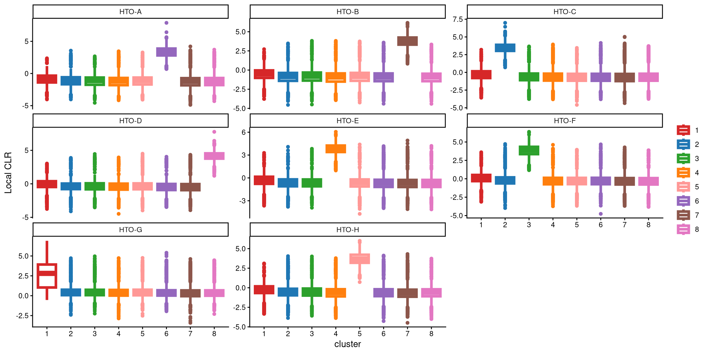
With 8 clusters, the expression of HTO-G in cluster 1 is not high enough compared to the other clusters. Therefore, we tried adding one more cluster in the next step. In the new round of clustering, the optional parameter is set to TRUE so that the optional workflow is performed to obtain more clusters, and we start by adding one extra cluster, which corresponds to the default value of extra_cluster.
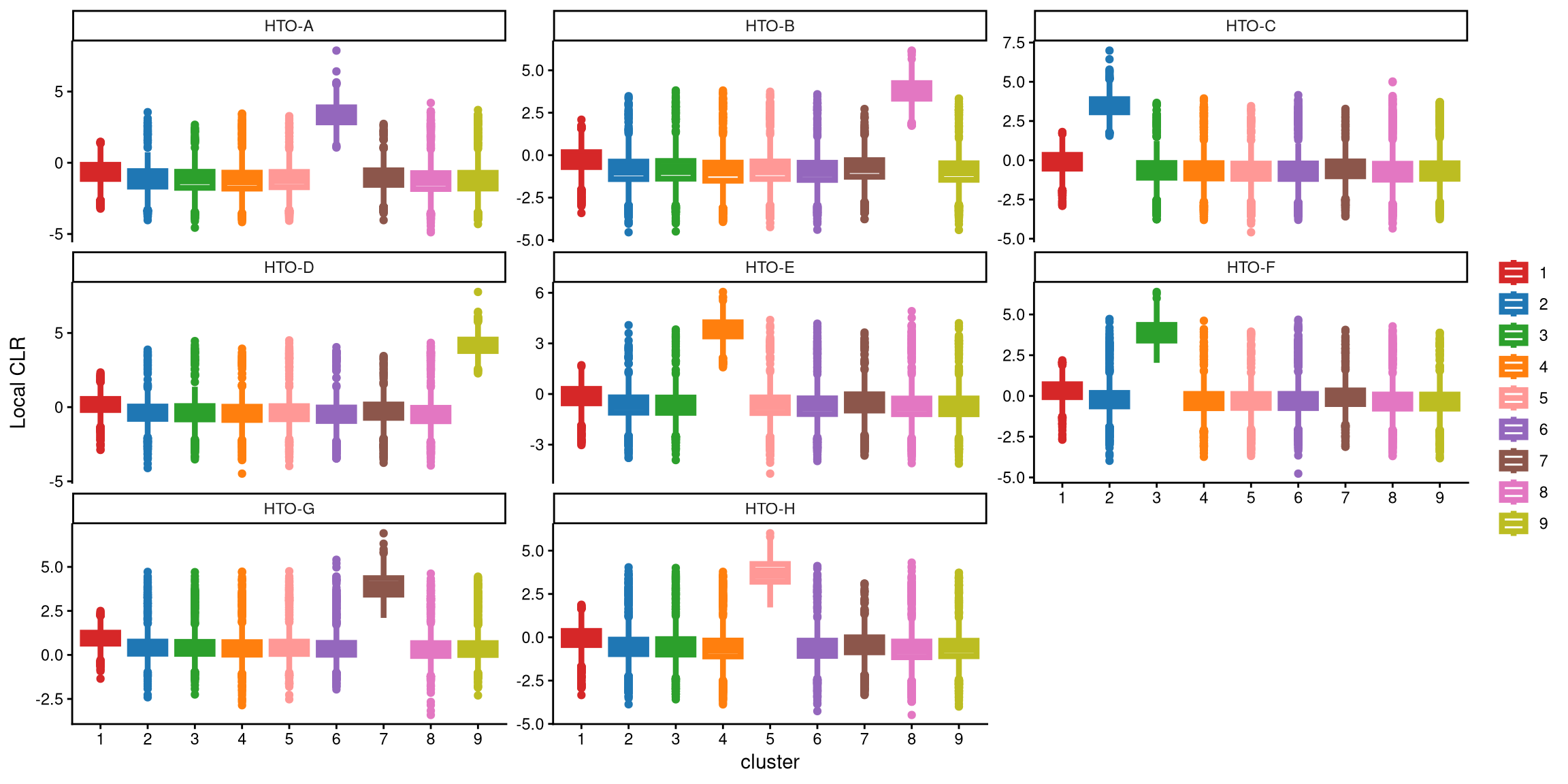
Compared to 8 clusters, 9 clusters better represent the data from different donors, and HTO-G is highly expressed in one cluster this time.
We use the following function to determine the optimal number of clusters to apply. Specifically, we calculate the CLR difference of the medians between 8 and 9 clusters for the maximum box in each HTO, and then select the HTO with the highest CLR difference. If this maximum CLR difference is greater than the cutoff (1), more clusters should be chosen.
## [1] "The largest CLR difference is:HTO-G 1.07. Choose optional clustering method (kmed.cl2 with9 clusters)."In this case, the median of cluster 1 in HTO-G for 8 clusters is 2.81, while the median of cluster 7 in HTO-G for 9 clusters is 3.88. Their difference is 1.07, which is larger than the default cutoff of 1, indicating that 9 clusters are better for this dataset.
Next, the Euclidean distance between cells and their corresponding cluster centroid within each cluster is calculated using EuclideanClusterDist.
12.3 Definition of non-core cells
Core cells are defined as cells that are closer to their cluster centroids, while non-core cells are those that are farther away from the cluster centroid. The cut-off between core and non-core cells can be determined using EuclideanDistPlot, which visualizes the cut-off based on the quantile of the distribution via the eu_cut_q parameter, shown as the red line in the plot. Each value in the eu_cut_q parameter corresponds to a cut-off for a cluster.
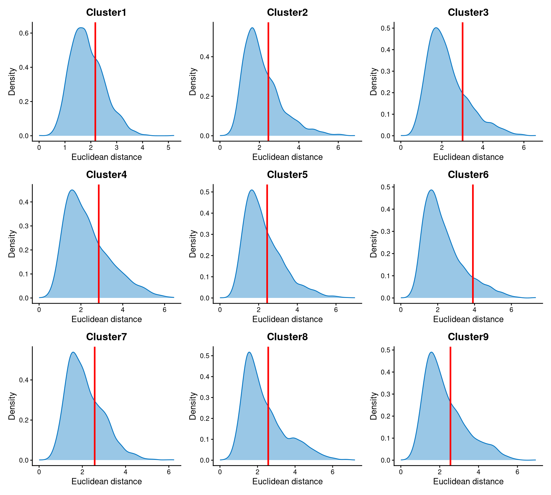
The Euclidean distances of each cluster are right-skewed, and the cut-off is set at the tail of each distribution.
Core and non-core cells are then classified using DefineNonCore, with eu_cut_q determined from the above plots. Since an optional extra cluster was added during the k-medoids clustering step, the optional parameter should be set to TRUE, and clr.norm should be supplied from the output of LocalCLRNorm.
pbmc.noncore <- DefineNonCore(pbmc.cl.dist, pbmc.kmed.cl2, eu_cut_q = c(0.7, 0.7, 0.8, 0.73, 0.65, 0.9, 0.72, 0.67, 0.67), optional = TRUE, clr.norm = pbmc.clr.norm)
table(pbmc.noncore)
## pbmc.noncore
## Cluster2 Cluster3 Cluster4 Cluster5 Cluster6 Cluster7 Cluster8 Cluster9 non-core
## 1727 1677 1567 1666 2388 1592 1941 1578 7386Core cells are labelled by their clusters, and non-core cells are directly labelled as “non-core.”
The definition of core and non-core cells is further examined using CLRPlot.
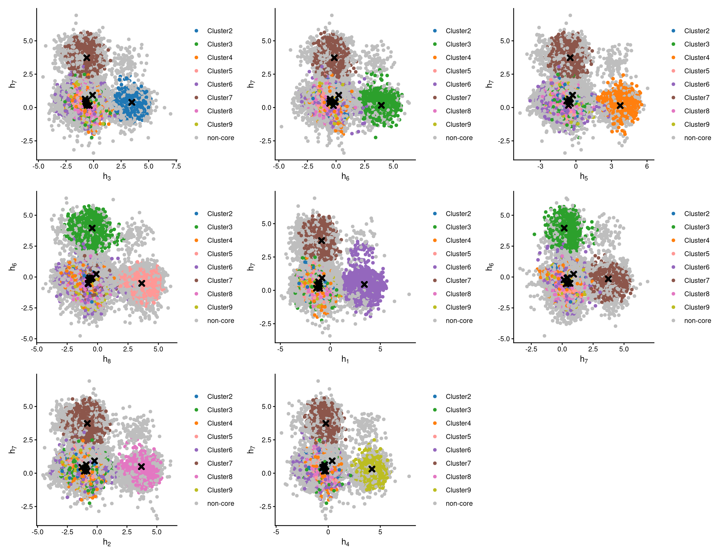
The pairwise local CLR-normalized values are shown in the above plots. Each plot clearly demonstrates two clusters, with other clusters appearing in the corners. Cluster centroids are indicated by cross symbols. Core cells cluster around the centroids, whereas non-core cells lie at the edges of the clusters.
12.4 Label clusters by sample
Each cluster will be labelled with its original sample, and here we use the default medoid-based labelling method.
pbmc.cluster.assign <- LabelClusterHTO(pbmc.clr.norm, pbmc.kmed.cl2, pbmc.noncore, label_method = "medoids")
pbmc.cluster.assign
## HTO-A HTO-B HTO-C HTO-D HTO-E HTO-F HTO-G HTO-H
## 6 8 2 9 4 3 7 5The results show each sample and its corresponding cluster index. For example, cluster 2 corresponds to the HTO-C sample. Cluster 1 does not correspond to any sample, and its cells are non-core cells.
12.5 Computing the Mahalanobis distance
Using the local CLR-normalized values from LocalCLRNorm, the non-core cell classifications from DefineNonCore, the k-medoids clustering from KmedCluster, and the cluster labelling from LabelClusterHTO, the Mahalanobis distance for each single cell can be calculated using CalculateMD.
pbmc.md.mat <- CalculateMD(pbmc.clr.norm, pbmc.noncore, pbmc.kmed.cl2, pbmc.cluster.assign)
pbmc.md.mat[,1:10]
## TGCCAAATCTCTAAGG ACTGCTCAGGTGTTAA TTCTTAGTCAACACGT CATTCGCCACAGTCGC TGGACGCCATCGACGC CGAGAAGTCAACTCTT ATGAGGGAGATGTTAG
## HTO-A 5.202772 10.253634 9.127812 7.145949 6.625931 8.884701 7.963672
## HTO-B 4.890115 7.446692 8.407859 6.612897 5.397583 6.459390 9.241414
## HTO-C 5.722017 4.113818 6.751875 5.855858 6.082566 5.675652 9.247818
## HTO-D 8.197005 11.199207 8.233957 5.767000 8.050543 8.688853 9.532406
## HTO-E 5.527910 9.810537 7.162078 7.245810 5.571156 6.013157 2.901250
## HTO-F 6.162433 10.771492 3.696816 6.165280 7.066276 5.633169 9.141619
## HTO-G 5.915178 9.915090 7.154785 5.153916 5.436461 6.425448 7.431548
## HTO-H 6.977708 9.760098 7.524617 5.475377 4.910284 6.832680 8.145188
## ACGCAGCCAAGCGCTC GACCTGGAGATCTGCT TAGTTGGAGGCTAGGT
## HTO-A 9.886572 5.690605 4.881149
## HTO-B 11.188029 8.554800 6.558717
## HTO-C 10.604653 5.316821 4.987928
## HTO-D 12.360201 6.881824 7.018003
## HTO-E 9.832322 6.098357 6.965630
## HTO-F 10.189380 7.193016 7.100530
## HTO-G 10.299582 6.953435 4.623985
## HTO-H 3.491173 5.138016 7.507943The output is a Mahalanobis distance matrix with rows representing hashtag samples and columns representing cells. Each entry indicates the Mahalanobis distance of a cell to a given hashtag sample.
12.6 Detect outlier cells
Outlier cells, including negatives and doublets, are defined based on the distribution of the minimum Mahalanobis distance across all cells, which can be visualized using MDDensPlot. The cut-off in the plot is determined by the md_cut_q parameter, which specifies the quantile of the distribution and is shown as the red line. Users are encouraged to adjust the cut-off through the md_cut_q parameter.
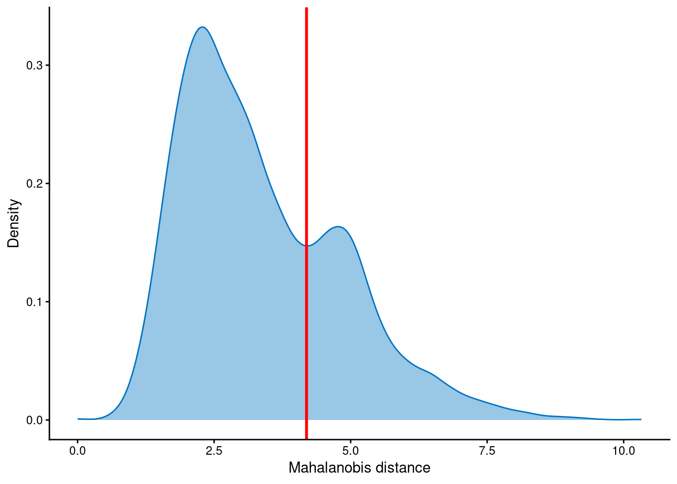
It is clear that the Mahalanobis distance is bimodally distributed: the peak with the smaller Mahalanobis distance corresponds to singlets, while the peak with the larger Mahalanobis distance corresponds to outlier cells. Therefore, the cut-off should be set at the anti-mode of the distribution.
Outlier cells are then defined using AssignOutlierDrop according to the cut-off selected from the plot.
## pbmc.outlier.assign
## Outlier Singlet
##    6026   15496
In this step, cells are labelled as either outliers or singlets.
12.7 Demultiplexing
The HTO library sizes are used to further distinguish negatives and doublets among the outlier cells. The distribution of HTO library sizes can be visualized using OutlierHTOPlot. The possible cut-offs corresponding to the modes and anti-modes are shown as red lines in the plot. The rest of the parameters are set as default values.
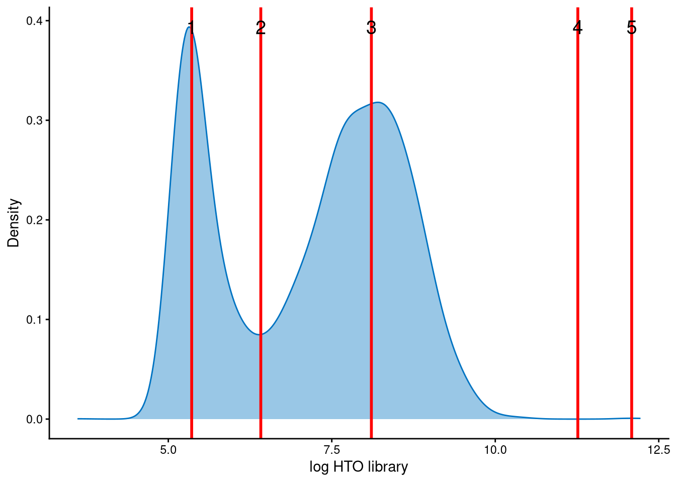
The distribution of HTO library sizes across outlier cells is classically bimodal, with a peak of smaller HTO library sizes corresponding to negatives and a peak of larger HTO library sizes corresponding to doublets. The cut-off should be set at the anti-mode of the distribution, which is line 2.
In the final step of demultiplexing, the Mahalanobis distance from CalculateMD, the original hashtag count matrix, the outlier classifications from AssignOutlierDrop, the gene expression data, and the selected HTO library size cut-off from the above plot are applied. Since optional clustering was applied to this dataset with extra clusters, optional is set to TRUE. K-medoids clustering from KmedCluster and the sample-label assignment from LabelClusterHTO are then applied to obtain the final demultiplexing results.
pbmc.cmddemux.assign <- CMDdemuxClass(pbmc.md.mat, pbmc.hash.count, pbmc.outlier.assign, use_gex_data = TRUE, gex.count = pbmc.gex.count, num_modes = 3, cut_no = 2, optional = TRUE, kmed.cl = pbmc.kmed.cl2, cluster.assign = pbmc.cluster.assign)
head(pbmc.cmddemux.assign)
## demux_id global_class demux_global_class doublet_class
## TGCCAAATCTCTAAGG HTO-B Negative Negative Negative
## ACTGCTCAGGTGTTAA HTO-C Singlet HTO-C HTO-C
## TTCTTAGTCAACACGT HTO-F Singlet HTO-F HTO-F
## CATTCGCCACAGTCGC HTO-G Negative Negative Negative
## TGGACGCCATCGACGC HTO-H Negative Negative Negative
## CGAGAAGTCAACTCTT HTO-F Negative Negative NegativeCMDdemux provides four types of outputs:
demux_id: the identity for each cell, determined by the sample with the minimum Mahalanobis distance for that cell.
global_class: classification of each cell as Singlet, Doublet, or Negative.
demux_global_class: singlet cells are labeled with their original sample, while negatives and doublets are labeled accordingly.
doublet_class: similar to demux_global_class, but doublets are labeled with their sample of origin. This is particularly useful for combined-hashtag experiments.
##
##  Doublet    HTO-A    HTO-B    HTO-C    HTO-D    HTO-E    HTO-F    HTO-G    HTO-H Negative
##     3054     2181     2322     2181     1952     1754     1785     2053     2174     2066
The output above shows the number of cells demultiplexed into each category.