Chapter 8 EMBRYO MULTI-Seq CMO
This dataset is low quality (Brown et al. 2024) and includes 19,494 cells from an embryonic day 18.5 mouse brain. All cells originate from a single mouse and were partitioned into 12 replicates labelled using MULTI-Seq cholesterol-modified oligos (CMOs). The low quality is due to contamination of CMOs, which results in a cluster of cells with moderate expression of all hashtags.
The subset of hash count data is shown below:
## 12 x 10 sparse Matrix of class "dgCMatrix"## [[ suppressing 10 column names 'AAACCCAAGATGCTTC-1', 'AAACCCAAGGTAAAGG-1', 'AAACCCAAGGTAAGAG-1' ... ]]##
## Nxt_451 100 2 5 3 23 55 9 1 19 28
## Nxt_452 5 8 4 7 145 277 40 . 113 40
## Nxt_453 7 1302 24 15 124 53 24 1 65 77
## Nxt_455 2 5 2 2 34 50 14 1 28 26
## Nxt_456 4 6 4 12 103 78 26 1 27 69
## Nxt_457 13 12 13 16 94 113 16 . 36 30
## Nxt_458 1 1 3 2 15 10 1 . 1 1
## Nxt_459 2 2 6 5 81 191 1348 . 85 8
## Nxt_460 12 15 17 1952 190 325 19 3 331 38
## Nxt_462 1 3 4 2 26 7 4 1 22 7
## Nxt_463 5 28 202 6 51 64 1 . 27 32
## Nxt_465 3 . . 2 25 11 1 . 8 6The subset of gene expression data is shown below:
## 10 x 10 sparse Matrix of class "dgCMatrix"## [[ suppressing 10 column names 'AAACCCAAGATGCTTC-1', 'AAACCCAAGGTAAAGG-1', 'AAACCCAAGGTAAGAG-1' ... ]]##
## Xkr4 . . . . . . . . . .
## Gm1992 . . . . . . . . . .
## Gm19938 . . . . . . . . . .
## Gm37381 . . . . . . . . . .
## Rp1 . . . . . . . . . .
## Sox17 . . . . . . . . . .
## Gm37587 . . . . . . . . . .
## Gm37323 . . . . . . . . . .
## Mrpl15 . 1 . 1 . . . . . .
## Lypla1 . . . . . . . 1 . .8.1 Local CLR normalization
The first step of CMDdemux is to normalize the hash count data using a local CLR normalization.
##         AAACCCAAGATGCTTC-1 AAACCCAAGGTAAAGG-1 AAACCCAAGGTAAGAG-1 AAACCCAAGTGGAAGA-1 AAACCCACACTTCTCG-1 AAACCCACAGAAGCGT-1
## Nxt_451         2.77667561        -1.07545594         -0.3009406         -0.8925163         -0.8786419        -0.04635267
## Nxt_452        -0.04668544         0.02315634         -0.4832622         -0.1993691          0.9269109         1.55591676
## Nxt_453         0.24099663         4.99835634          1.1261758          0.4937781          0.7716180        -0.08272031
## Nxt_455        -0.73983262        -0.38230876         -0.9940878         -1.1801984         -0.5013477        -0.13987872
## Nxt_456        -0.22900700        -0.22815808         -0.4832622          0.2861387          0.5876952         0.29774350
## Nxt_457         0.80061242         0.39088112          0.5463573          0.5544027          0.4971812         0.66449409
## Nxt_458        -1.14529773        -1.48092105         -0.7064057         -1.1801984         -1.2841070        -1.67380908
## Nxt_459        -0.73983262        -1.07545594         -0.1467899         -0.4870512          0.3500235         1.18579102
## Nxt_460         0.72650445         0.59852049          0.7976717          5.2983113          1.1955777         1.71519303
## Nxt_462        -1.14529773        -0.78777387         -0.4832622         -1.1801984         -0.7608588        -1.99226281
## Nxt_463        -0.04668544         1.19322760          3.2205059         -0.3329005         -0.1054520         0.10268291
## Nxt_465        -0.45215055        -2.17406823         -2.0927001         -1.1801984         -0.7985992        -1.58679771
##         AAACCCACATTGCCGG-1 AAACCCAGTACAGAAT-1 AAACCCAGTATTAAGG-1 AAACCCAGTCGAGATG-1
## Nxt_451        -0.36107024          0.2888113         -0.4917308          0.3263218
## Nxt_452         1.04991674         -0.4043359          1.2487354          0.6725980
## Nxt_453         0.55522049          0.2888113          0.7021917          1.3157348
## Nxt_455         0.04439487          0.2888113         -0.1201672          0.2548628
## Nxt_456         0.63218153          0.2888113         -0.1552585          1.2075212
## Nxt_457         0.16955801         -0.4043359          0.1234549          0.3930131
## Nxt_458        -1.97050815         -0.4043359         -2.7943159         -2.3478269
## Nxt_459         4.54346352         -0.4043359          0.9668843         -0.8437495
## Nxt_460         0.33207694          0.9819585          2.3176719          0.6225876
## Nxt_462        -1.05421742          0.2888113         -0.3519688         -0.9615325
## Nxt_463        -1.97050815         -0.4043359         -0.1552585          0.4555335
## Nxt_465        -1.97050815         -0.4043359         -1.2902385         -1.0950639
The output of LocalCLRNorm is a normalized data matrix with rows representing hashtag samples and columns representing cells. Each entry is a normalized value.
8.2 K-medoids clustering
The local CLR-normalized values are used here for K-medoids clustering. Since this dataset has twelve samples, the default parameters are initially applied, which divide the cells into twelve clusters.
We use a boxplot to check whether the number of clusters is appropriate for clustering. An ideal result is that one box should be significantly higher than the other boxes in each panel.
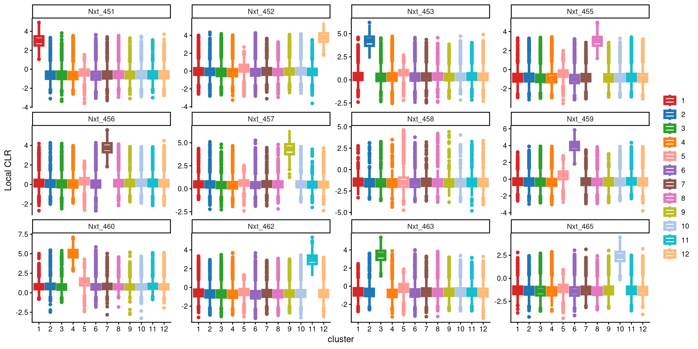
From this plot, it is clear that the hash Nxt_458 does not distinguish 12 clusters, as its expression is similar across all twelve clusters. Therefore, additional clusters are needed.
In the updated clustering workflow, the optional parameter is set to TRUE, which enables the optional step for adding extra clusters. The extra_cluster parameter specifies the number of additional clusters to include. Here, we start by adding one extra cluster.
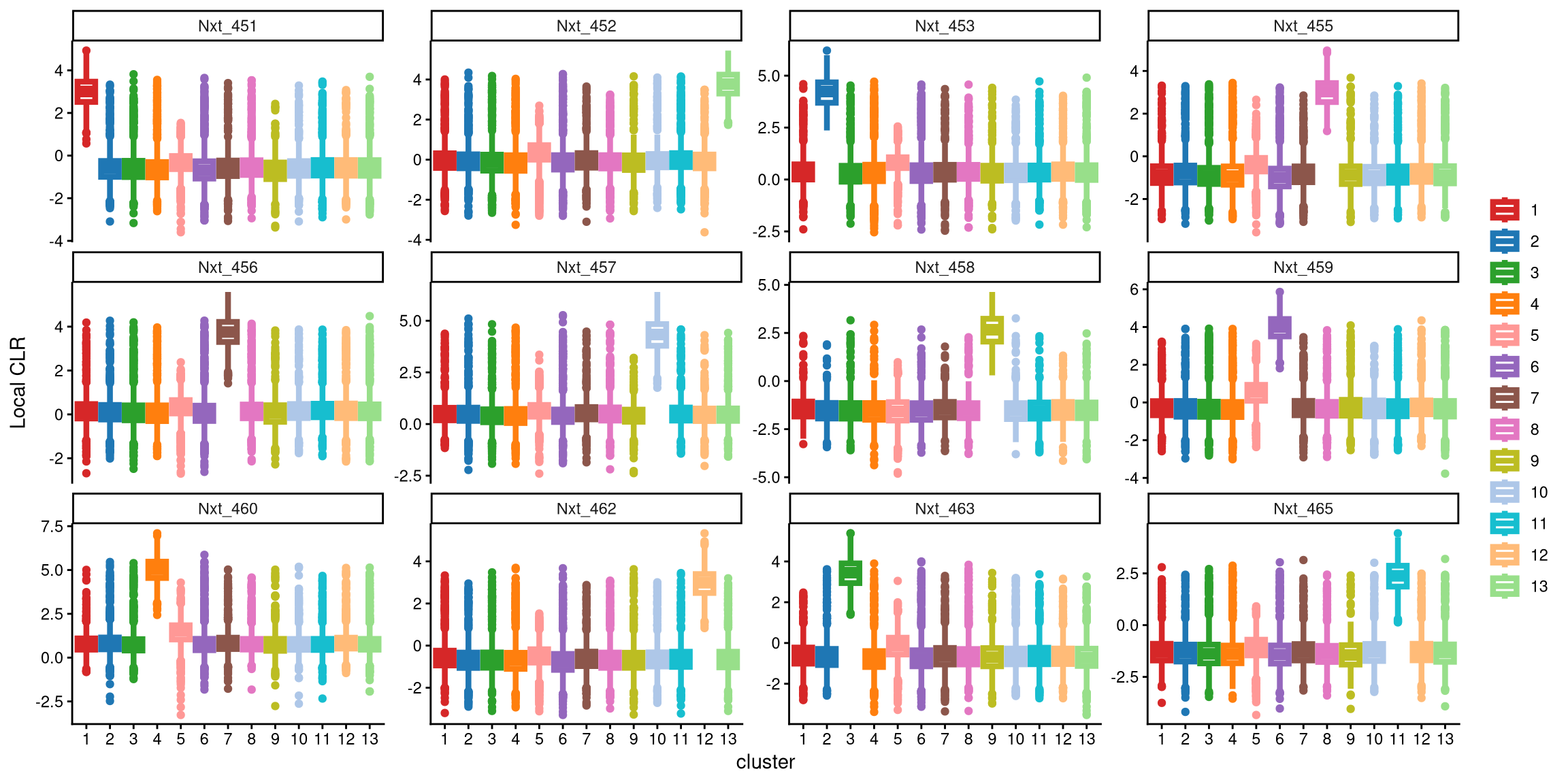
After applying 13 clusters, each CMO is uniquely and highly expressed in one cluster, indicating that 13 clusters are appropriate for this dataset.
The ExamineClusterNumber function can then be used to further assess whether 12 or 13 clusters are more suitable. For each hashtag, the difference between the median value of the largest box in the plot with 13 clusters and that in the plot with 12 clusters is compared with the cut-off defined by the fc_cut parameter. The default parameter is recommended. The underlying idea is that if additional clusters are appropriate, the hashtag should show a higher expression in one of the additional clusters; if not, the expression pattern will remain similar. Thus, setting a threshold based on the difference in median CLR values between the largest boxes for the two cluster numbers helps determine the appropriate number of clusters.
## [1] "The largest CLR difference is:Nxt_458 4.085. Choose optional clustering method (kmed.cl2 with13 clusters)."In this case, with 13 clusters, Nxt_458 is highly and uniquely expressed in cluster 9, whereas with 12 clusters, it is maximally expressed in cluster 1. The difference between the median values of these two clusters is 4.058, which exceeds the default cut-off of 1. Therefore, 13 clusters are recommended for this dataset.
Next, the Euclidean distance between cells and their corresponding cluster centroid within each cluster is calculated using EuclideanClusterDist.
8.3 Definition of non-core cells
Core cells are defined as cells that are closer to their cluster centroids, while non-core cells are those that are farther away from the cluster centroid. The cut-off between core and non-core cells can be determined using EuclideanDistPlot, which visualizes the cut-off based on the quantile of the distribution via the eu_cut_q parameter, shown as the red line in the plot. Each value in the eu_cut_q parameter corresponds to a cut-off for a cluster.
EuclideanDistPlot(emcmo.cl.dist, eu_cut_q = c(0.9, 0.81, 0.81, 0.79, 0.23, 0.72, 0.95, 0.84, 0.83, 0.9, 0.8, 0.91, 0.79))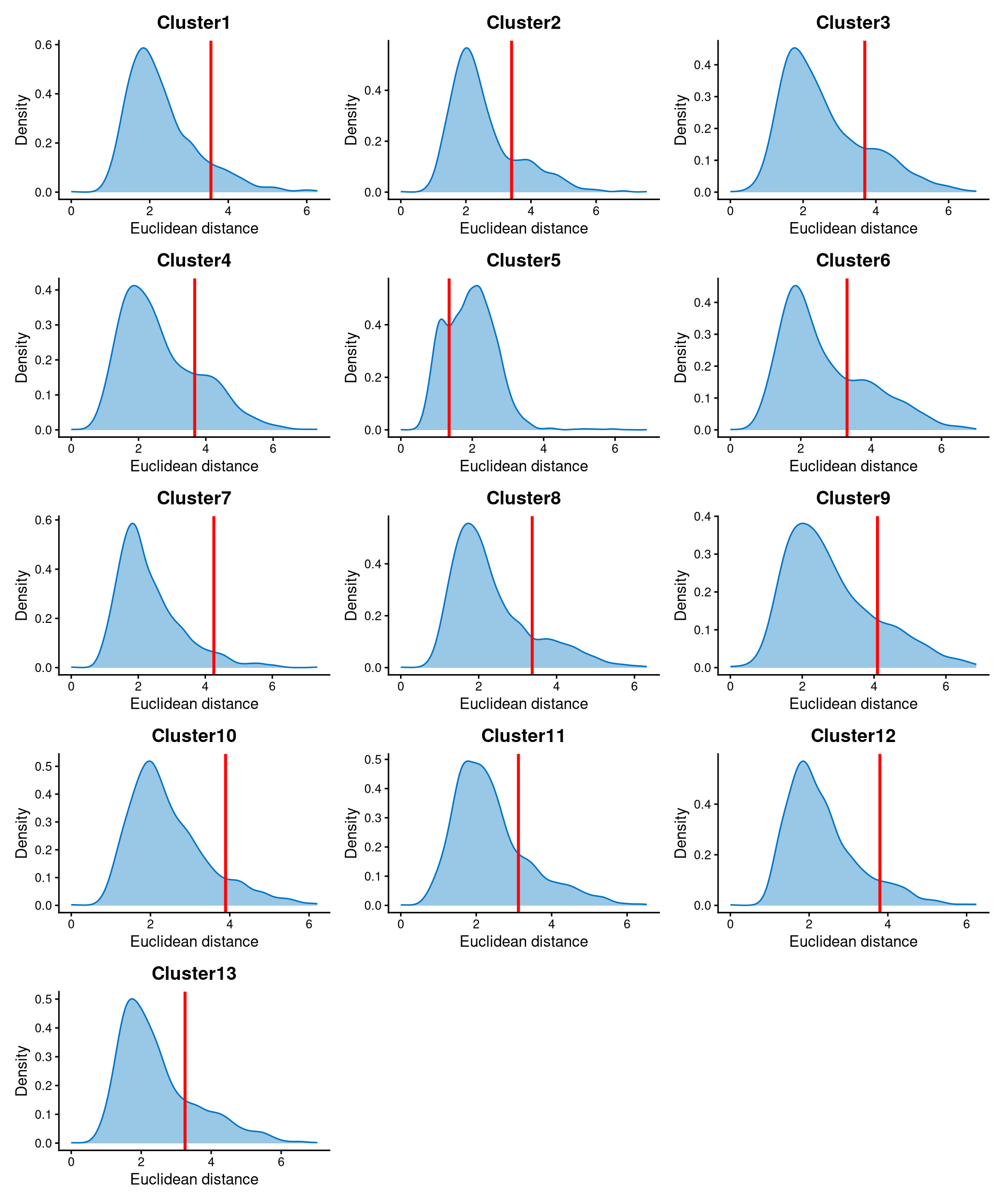
For most clusters, the Euclidean distance is bimodally distributed, and the cut-off can be set at the anti-mode of the distribution. Cells with Euclidean distance greater than the cluster-specific cut-off are defined as non-core cells, while the remaining cells are defined as core cells.
Core and non-core cells are then classified using DefineNonCore, with eu_cut_q determined from the above plots. Since an optional extra cluster was added during the k-medoids clustering step, the optional parameter should be set to TRUE, and clr.norm should be supplied from the output of LocalCLRNorm.
emcmo.noncore <- DefineNonCore(emcmo.cl.dist, emcmo.kmed.cl2, eu_cut_q = c(0.9, 0.81, 0.81, 0.79, 0.23, 0.72, 0.95, 0.84, 0.83, 0.9, 0.8, 0.91, 0.79), optional = TRUE, clr.norm = emcmo.clr.norm)
table(emcmo.noncore)
## emcmo.noncore
## Cluster1 Cluster10 Cluster11 Cluster12 Cluster13 Cluster2 Cluster3 Cluster4 Cluster6 Cluster7 Cluster8 Cluster9 non-core
## 1154 796 1009 1130 1061 1004 1066 1071 1115 1157 1145 416 7370Core cells are labelled by their clusters, and non-core cells are directly labelled as “non-core.”
The definition of core and non-core cells is further examined using CLRPlot.
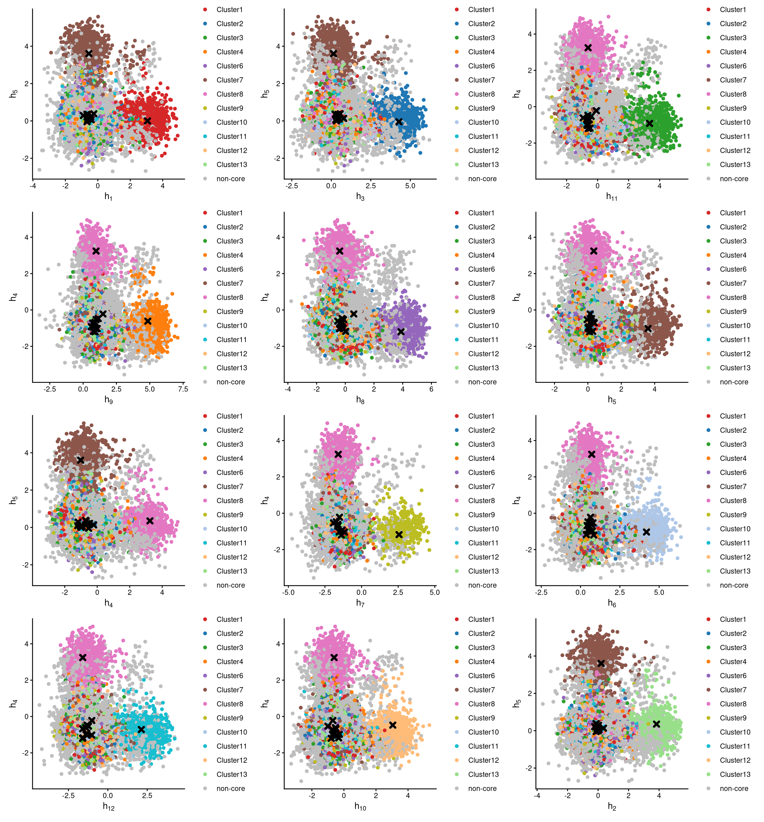
The pairwise local CLR-normalized values are shown in the above plots. Each plot clearly demonstrates two clusters, with other clusters appearing in the corners. Cluster centroids are indicated by cross symbols. All cells in cluster 5 are defined as non-core cells. Because one extra cluster was added during clustering, there should be exactly one cluster of cells defined as non-core.
If we go back to the plot of Euclidean distance, the distribution of cluster 5 is somewhat unusual compared with the others, because all cells in cluster 5 are non-core cells. Therefore, the cut-off is not important, as the entire cluster 5 is defined as non-core.
8.4 Label clusters by sample
Each cluster will be labelled with its original sample, and here we use the alternative labelling method, “expression”. The expression-based labelling method can be explained using the plot from CheckCLRBoxPlot. Each hashtag sample is assigned to the cluster whose box has the maximum median local CLR value. For example, Nxt_451 is highly expressed in cluster 1 compared with the other clusters; therefore, cluster 1 corresponds to the Nxt_451 sample.
emcmo.cluster.assign <- LabelClusterHTO(emcmo.clr.norm, emcmo.kmed.cl2, emcmo.noncore, label_method = "expression")
emcmo.cluster.assign
## Nxt_451 Nxt_452 Nxt_453 Nxt_455 Nxt_456 Nxt_457 Nxt_458 Nxt_459 Nxt_460 Nxt_462 Nxt_463 Nxt_465
## 1 13 2 8 7 10 9 6 4 12 3 11The results show each sample and its corresponding cluster index. For example, cluster 2 corresponds to the Nxt_453 sample. Cluster 5 does not correspond to any sample, and its cells are non-core cells.
8.5 Computing the Mahalanobis distance
Using the local CLR-normalized values from LocalCLRNorm, the non-core cell classifications from DefineNonCore, the k-medoids clustering from KmedCluster, and the cluster labelling from LabelClusterHTO, the Mahalanobis distance for each single cell can be calculated using CalculateMD.
emcmo.md.mat <- CalculateMD(emcmo.clr.norm, emcmo.noncore, emcmo.kmed.cl2, emcmo.cluster.assign)
emcmo.md.mat[,1:10]
## AAACCCAAGATGCTTC-1 AAACCCAAGGTAAAGG-1 AAACCCAAGGTAAGAG-1 AAACCCAAGTGGAAGA-1 AAACCCACACTTCTCG-1 AAACCCACAGAAGCGT-1
## Nxt_451 2.341772 10.220819 7.825469 9.635047 6.436948 6.564476
## Nxt_452 8.209578 9.461707 8.583488 9.705580 4.793082 5.009615
## Nxt_453 8.355703 3.606572 7.775431 9.615081 5.904429 8.032104
## Nxt_455 8.033499 9.553399 8.527194 9.697020 5.842976 6.379291
## Nxt_456 8.161931 10.350754 8.885066 8.772574 5.309745 6.801436
## Nxt_457 8.034306 10.264371 8.412973 9.803269 6.985292 7.871071
## Nxt_458 8.517906 9.948915 7.709101 9.587891 6.384782 7.903263
## Nxt_459 8.560238 10.678996 8.552979 9.798039 5.685747 5.619522
## Nxt_460 8.712636 10.907609 9.490306 2.026628 6.655323 6.906002
## Nxt_462 8.372702 9.740508 8.118033 9.564131 6.173018 8.459722
## Nxt_463 7.044443 8.269705 2.262769 9.702226 5.656728 6.538878
## Nxt_465 6.144202 9.572345 8.436082 9.063390 5.024707 7.233999
## AAACCCACATTGCCGG-1 AAACCCAGTACAGAAT-1 AAACCCAGTATTAAGG-1 AAACCCAGTCGAGATG-1
## Nxt_451 9.429873 5.466845 6.931293 5.877465
## Nxt_452 8.452728 7.160642 5.189715 6.007992
## Nxt_453 9.827031 7.346923 6.970200 5.855915
## Nxt_455 9.010376 5.546704 6.440718 5.709187
## Nxt_456 8.970280 6.278943 7.241708 5.566265
## Nxt_457 10.681242 8.455316 8.488461 8.183124
## Nxt_458 10.116792 6.054657 9.151608 8.638527
## Nxt_459 3.955615 7.448448 6.224253 8.052452
## Nxt_460 10.959526 7.324837 5.781487 8.081393
## Nxt_462 9.878995 5.412398 6.385911 7.013540
## Nxt_463 11.077002 6.551475 6.992089 5.528224
## Nxt_465 9.987046 5.010392 6.721998 5.737517The output is a Mahalanobis distance matrix with rows representing hashtag samples and columns representing cells. Each entry indicates the Mahalanobis distance of a cell to a given hashtag sample.
8.6 Detect outlier cells
Outlier cells, including negatives and doublets, are defined based on the distribution of the minimum Mahalanobis distance across all cells, which can be visualized using MDDensPlot. The cut-off in the plot is determined by the md_cut_q parameter, which specifies the quantile of the distribution and is shown as the red line. Users are encouraged to adjust the cut-off through the md_cut_q parameter.
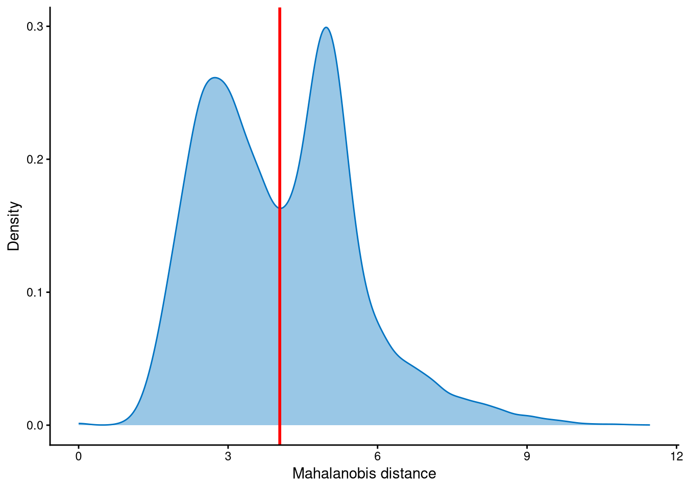
It is clear that the Mahalanobis distance is bimodally distributed in this dataset, so the cut-off is selected at the anti-mode of the distribution. The md_cut_q is set to 0.51, which means that 51% of cells are classified as singlets and the remaining 49% are classified as outlier cells. Most of these outlier cells correspond to cells in the contaminated cluster, which will be explained later.
Outlier cells are then defined using AssignOutlierDrop according to the cut-off selected from the plot.
emcmo.outlier.assign <- AssignOutlierDrop(emcmo.md.mat,  md_cut_q = 0.51)
table(emcmo.outlier.assign)
## emcmo.outlier.assign
## Outlier Singlet
## 9552 9942In this step, cells are labelled as either outliers or singlets.
8.7 Demultiplexing
The HTO library sizes are used to further distinguish negatives and doublets among the outlier cells. The distribution of HTO library sizes can be visualized using OutlierHTOPlot. The possible cut-offs corresponding to the modes and anti-modes are shown as red lines in the plot. The parameter num_modes is used to set the number of modes in the plot.
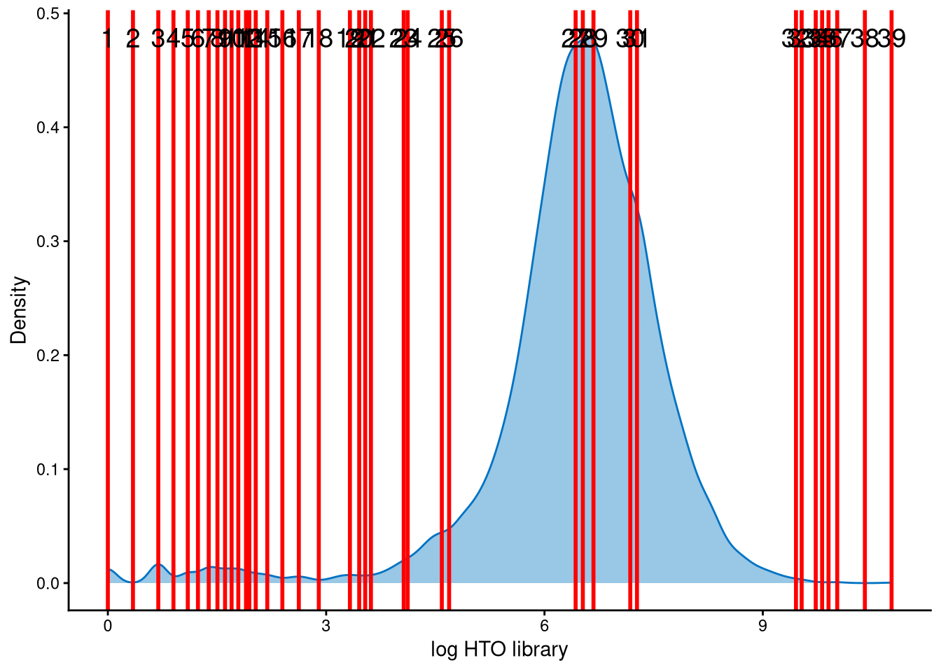
The distribution of HTO library sizes for these outlier cells is not typically multimodal, so a large value of num_modes was tested to identify an appropriate cut-off between negatives and doublets. Lines 25 and 26 are considered possible cut-offs because their values are close to 5, which corresponds to an HTO library size (total hashtag counts per cell) of \(e^5\approx148\), a reasonable threshold. We ultimately choose line 26 as the cut-off.
In the final step of demultiplexing, the Mahalanobis distance from CalculateMD, the original hashtag count matrix, the outlier classifications from AssignOutlierDrop, the gene expression data, and the selected HTO library size cut-off from the above plot are applied.
emcmo.cmddemux.assign <- CMDdemuxClass(emcmo.md.mat, emcmo.hash.count, emcmo.outlier.assign, use_gex_data = TRUE, gex.count = emcmo.gex.count, num_modes = 20, cut_no = 26)
head(emcmo.cmddemux.assign)
## demux_id global_class demux_global_class doublet_class
## AAACCCAAGATGCTTC-1 Nxt_451 Singlet Nxt_451 Nxt_451
## AAACCCAAGGTAAAGG-1 Nxt_453 Singlet Nxt_453 Nxt_453
## AAACCCAAGGTAAGAG-1 Nxt_463 Singlet Nxt_463 Nxt_463
## AAACCCAAGTGGAAGA-1 Nxt_460 Singlet Nxt_460 Nxt_460
## AAACCCACACTTCTCG-1 Nxt_452 Doublet Doublet Nxt_452_Nxt_465
## AAACCCACAGAAGCGT-1 Nxt_452 Singlet Nxt_452 Nxt_452CMDdemux provides four types of outputs:
demux_id: the identity for each cell, determined by the sample with the minimum Mahalanobis distance for that cell.
global_class: classification of each cell as Singlet, Doublet, or Negative.
demux_global_class: singlet cells are labeled with their original sample, while negatives and doublets are labeled accordingly.
doublet_class: similar to demux_global_class, but doublets are labeled with their sample of origin. This is particularly useful for combined-hashtag experiments.
##
##  Doublet Negative     OT-E     OT-F     OT-G     OT-H
##      799       17     1211     1445     3861     2072
The output above shows the number of cells demultiplexed into each category.
8.8 The contaminated cluster
Figure 8.1 demonstrates the contaminated cluster. Fig. 8.1a,b show that cluster 5 is a large cluster that includes negatives, doublets, and singlets from different samples, and this cluster is the contaminated cluster. This indicates that 13 clusters are needed for this dataset, and the extra cluster (cluster 5) is defined as non-core cells according to the output of LabelClusterHTO. Since the cells in this cluster are far away from the cluster centroids of all other clusters, their Mahalanobis distances are larger. Therefore, it is not surprising to observe a bimodal distribution of Mahalanobis distances in MDDensPlot, where most cells with the larger-distance peak correspond to the contaminated cluster 5. In addition, the log raw hashtag counts for each hashtag are trimodally distributed (Fig. 8.1c). The second peak of each hashtag corresponds to the contaminated cluster, which shows moderate expression of each hashtag, higher than negatives but lower than singlets, and is considered a contaminated signal.
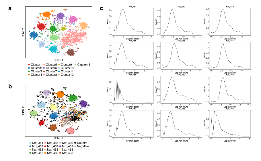
Figure 8.1: The contaminated cluster in the EMBRYO MULTI-Seq CMO dataset. (a) K-medoids clustering. (b) CMDdemux demultiplexing. (c) Distribution of log-transformed raw counts of each hashtag.
8.9 Examination of suspicious droplets
In the original paper, HTODemux assigns more doublets and negatives to the contaminated cluster 5 compared to CMDdemux. We can use the functions CheckAssign2DPlot and CheckAssign3DPlot to visually assess whether the CMDdemux assignments are correct.
CheckAssign2DPlot consists of pairwise 2D plots of HTO library sizes, mRNA library sizes, the second Mahalanobis distance, and the ratio of the first to the second Mahalanobis distance. Negatives, singlets, and doublets are separated into different regions in these 2D plots.
CheckAssign3DPlot uses HTO library sizes, mRNA library sizes, and the ratio of the first to the second Mahalanobis distance to visualize negatives, singlets, and doublets in 3D.
First, apply HTODemux to the data.
emcmo.obj <- CreateSeuratObject(counts = emcmo.hash.count)
emcmo.obj[["HTO"]] <- CreateAssayObject(counts = emcmo.hash.count)
emcmo.obj <- NormalizeData(emcmo.obj, assay = "HTO", normalization.method = "CLR")
emcmo.obj <- HTODemux(emcmo.obj, assay = "HTO", positive.quantile = 0.99, verbose = FALSE)
Next, we randomly select 30 cells that are classified as doublets by HTODemux but as singlets by CMDdemux in the contaminated cluster 5. The selected cell barcodes are shown below.
emcmo.cl5.barcode <- names(emcmo.kmed.cl2$clustering)[which(emcmo.kmed.cl2$clustering %in% 5)]
emcmo.extra.doublet <- intersect(rownames(emcmo.cmddemux.assign)[which(emcmo.cmddemux.assign$global_class == "Singlet")], names(emcmo.obj$HTO_classification.global)[which(emcmo.obj$HTO_classification.global == "Doublet")])
emcmo.extra.doublet <- intersect(emcmo.extra.doublet, emcmo.cl5.barcode)
set.seed(2026)
barcode.random.idx1 <- sample(1:length(emcmo.extra.doublet), 30, replace = FALSE)
We then use CheckAssign2DPlot to visualize these cells in 2D.
CheckAssign2DPlot(emcmo.hash.count, emcmo.gex.count, emcmo.md.mat, cmddemux.assign = emcmo.cmddemux.assign, check_barcodes = emcmo.extra.doublet[barcode.random.idx1], check_barcode_size = 3)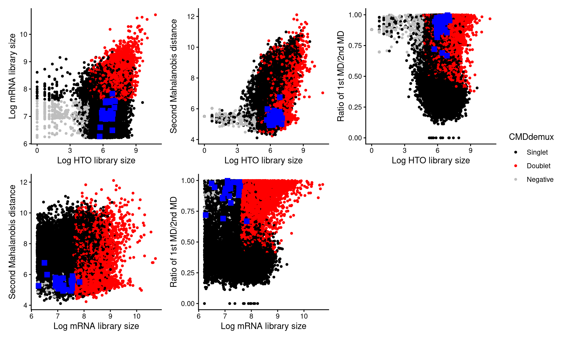
The randomly selected 30 cells are shown as blue squares in the plots. It is clear that most of these cells fall within the singlet region.
Alternatively, we can visualize these cells using the 3D plot from CheckAssign3DPlot.
CheckAssign3DPlot(emcmo.hash.count, emcmo.gex.count, emcmo.md.mat, cmddemux.assign = emcmo.cmddemux.assign, check_barcodes = emcmo.extra.doublet[barcode.random.idx1])In the 3D plot, the 30 cells are shown as blue points. The conclusion remains the same: most of the cells classified as doublets by HTODemux are actually singlets, and CMDdemux assigns them correctly.
We also examine cells classified as negatives by HTODemux but as singlets by CMDdemux in the contaminated cluster 5. Another 30 such cells are randomly selected, as shown below.
emcmo.extra.negative <- intersect(rownames(emcmo.cmddemux.assign)[which(emcmo.cmddemux.assign$global_class == "Singlet")], names(emcmo.obj$HTO_classification.global)[which(emcmo.obj$HTO_classification.global == "Negative")])
emcmo.extra.negative <- intersect(emcmo.extra.negative, emcmo.cl5.barcode)
set.seed(2026)
barcode.random.idx2 <- sample(1:length(emcmo.extra.negative), 30, replace = FALSE)
These extra negatives can be examined using CheckAssign2DPlot.
CheckAssign2DPlot(emcmo.hash.count, gex.count = emcmo.gex.count, emcmo.md.mat, cmddemux.assign = emcmo.cmddemux.assign, check_barcodes = emcmo.extra.negative[barcode.random.idx2], check_barcodes_col = "green", check_barcode_size = 3)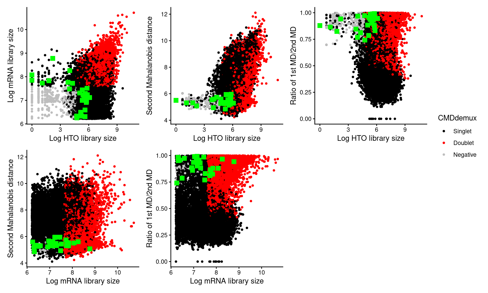
The randomly selected 30 cells are shown as green squares in the plots, and most of them also fall within the singlet region.
We then use CheckAssign3DPlot to inspect these cells in 3D.
CheckAssign3DPlot(emcmo.hash.count, emcmo.gex.count, emcmo.md.mat, cmddemux.assign = emcmo.cmddemux.assign, check_barcodes = emcmo.extra.negative[barcode.random.idx2], check_barcodes_col = "green")In the 3D plot, most droplets classified as negatives by HTODemux but as singlets by CMDdemux are mixed with singlets. Again, this supports the demultiplexing results from CMDdemux.