12.6 直方图
直方图用来查看连续变量的分布
ggplot(diamonds, aes(price)) + geom_histogram(bins = 30)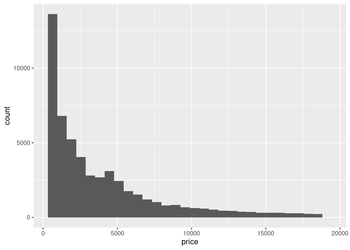
图 12.32: 钻石价格的分布
堆积直方图
ggplot(diamonds, aes(x = price, fill = cut)) + geom_histogram(bins = 30)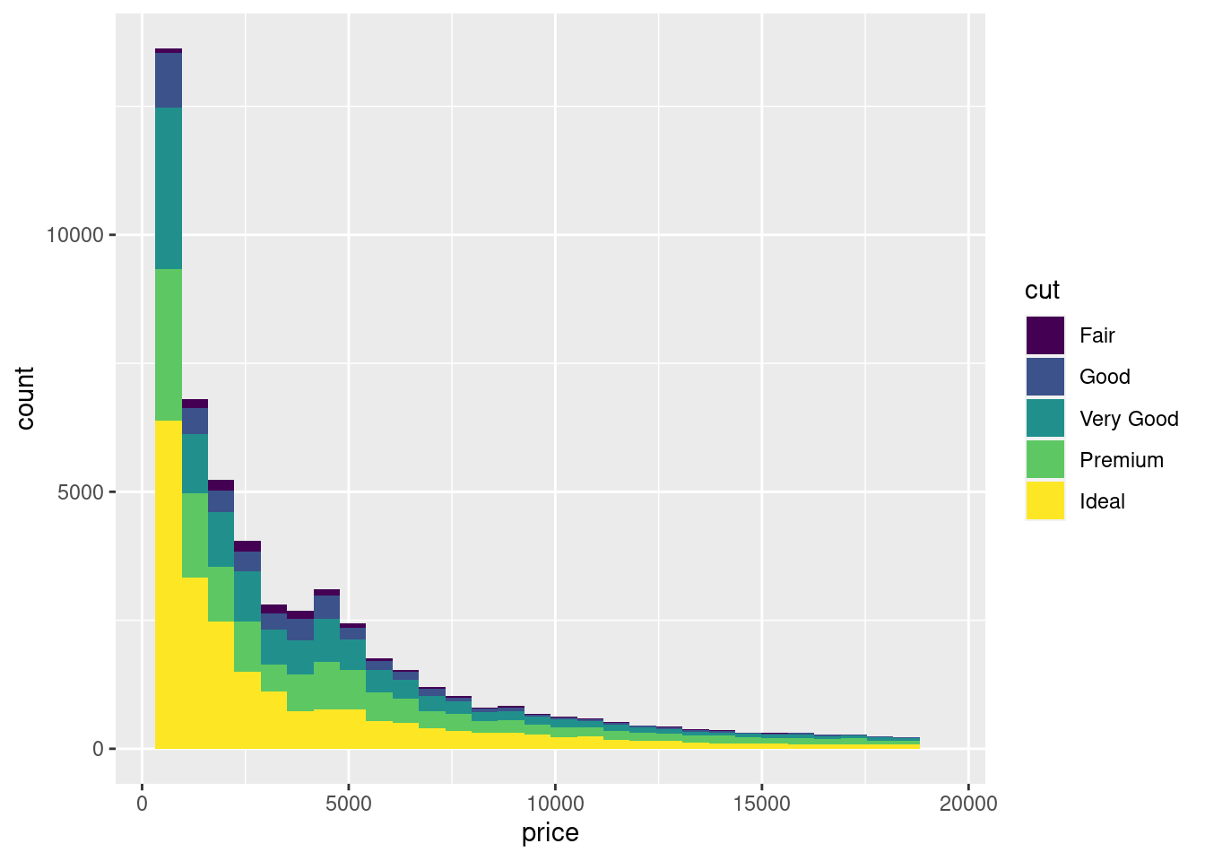
图 11.18: 钻石价格随切割质量的分布
基础 R 包与 Ggplot2 包绘制的直方图的对比,Base R 绘图速度快,代码更加稳定,Ggplot2 代码简洁,更美观
par(mar = c(2.1, 2.1, 1.5, 0.5))
plot(c(50, 350), c(0, 10),
  type = "n", font.main = 1,
  xlab = "", ylab = "", frame.plot = FALSE, axes = FALSE,
  # xlab = "hp", ylab = "Frequency",
  main = paste("Histogram with Base R", paste(rep(" ", 60), collapse = ""))
)
axis(
  side = 1, at = seq(50, 350, 50), labels = seq(50, 350, 50),
  tick = FALSE, las = 1, padj = 0, mgp = c(3, 0.1, 0)
)
axis(
  side = 2, at = seq(0, 10, 2), labels = seq(0, 10, 2),
  # col = "white", 坐标轴的颜色
  # col.ticks 刻度线的颜色
  tick = FALSE, # 取消刻度线
  las = 1, # 水平方向
  hadj = 1, # 右侧对齐
  mgp = c(3, 0.1, 0) # 纵轴边距线设置为 0.1
)
abline(h = seq(0, 10, 2), v = seq(50, 350, 50), col = "gray90", lty = "solid")
abline(h = seq(1, 9, 2), v = seq(75, 325, 50), col = "gray95", lty = "solid")
hist(mtcars$hp,
  col = "#56B4E9", border = "white",
  freq = TRUE, add = TRUE
  # labels = TRUE, axes = TRUE, ylim = c(0, 10.5),
  # xlab = "hp",main = "Histogram with Base R"
)
mtext("hp", 1, line = 1.0)
mtext("Frequency", 2, line = 1.0)

ggplot(mtcars) +
  geom_histogram(aes(x = hp), fill = "#56B4E9", color = "white", breaks = seq(50, 350, 50)) +
  scale_x_continuous(breaks = seq(50, 350, 50)) +
  scale_y_continuous(breaks = seq(0, 12, 2)) +
  labs(x = "hp", y = "Frequency", title = "Histogram with Ggplot2") +
  theme_minimal(base_size = 12)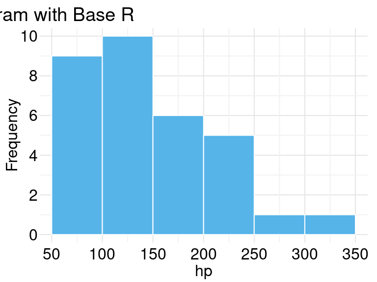
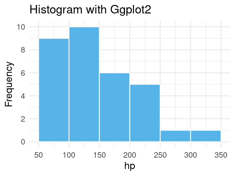
图 12.33: 直方图