Chapter 1 Variable Subset Selection

Consider the standard linear model: $$y = \beta_0 + \beta_1x_1 + \beta_2x_2 + \ldots + \beta_p x_p +\epsilon$$ Here, $y$ is the response variable, the $x$’s are the predictor variables and $\epsilon$ is an error term.

Subset selection involves identifying a subset of the $p$ predictors $x_1,...,x_p$ of size $d$ that we believe to be related to the response. We then fit a least squares linear regression model using just the reduced set of variables.

For example, if we believe that only $x_1$ and $x_2$ are related to the response, then we may take $d=2$ and fit a model of the following form: $$y = \beta_0 + \beta_1x_1 + \beta_2x_2 +\epsilon$$ where we have deemed variables $x_3,...,x_p$ to be irrelevant.

But how do we determine which variables are relevant? We may just `know’ which variables are most informative for a particular response (for example, from previous data investigations or talking to an expert in the field), but often we need to investigate.

How many possible linear models are we trying to choose from? Well, we will always include the intercept term $\beta_0$. Then each variable $X_1,...,X_p$ can either be included or not, hence we have $2^p$ possible models to choose from.

Question: how do we choose which variables should be included in our model?

1.1 Validation by Prediction Error

Much of the material in this section should be a refresher of validation techniques which you have seen in previous modules.

1.1.1 Training Error

The training error of a linear model is evaluated via the Residual Sum of Squares (RSS), which as we have seen is given by $$RSS = \sum_{i=1}^{n}(y_i - \hat{y}_i)^2,$$ where $$\hat{y}_i = \hat{\beta}_0+\hat{\beta}_1x_{i1} + \hat{\beta}_2x_{i2}+ \ldots + \hat{\beta}_dx_{id}.$$ is the predicted response value at input $x_i = (x_{i1},...,x_{id})$. Another very common metric is the Mean Squared Error (MSE) which is simply a scaled down version of $RSS$: $$MSE = \frac{RSS}{n}$$ where $n$ is the size of the training sample. Unfortunately, neither of these metrics is appropriate when comparing models of different dimensionality (different number of predictors) because both $RSS$ and $MSE$ generally decrease as we include additional predictors to a linear model.
In fact, in the extreme case of $n=p$ both metrics will be 0! This does not mean that we have a “good” model, just that we have overfitted our linear model to perfectly adjust to the training data. Overfitted models exhibit poor predictive performance (low training error but high prediction error). Our aim is to have simple, interpretable models with relatively small $p$ (in relation to $n$), which have good predictive performance.

1.1.2 Validation

Validation involves keeping a subset of the available data separate for the purposes of calculating a prediction error (otherwise called a test error):

1. Split the data into a training sample of size $n_T$ and a test/validation sample of size $n^*$ (note: $n = n_T + n^*$).
2. Train the model using the training sample to get $\hat{\beta}_0,\hat{\beta}_1,\ldots,\hat{\beta}_d$.
3. Use the validation sample to get predictions: $\hat{y}^*= \hat{\beta}_0+\hat{\beta}_1x_1^*+\ldots+\hat{\beta}_dx_d^*$.
4. Calculate the validation $RSS=\sum_{i=1}^{n^*}(y_i^*-\hat{y}_i^*)^2$.

• This procedure can be performed for all possible models and the model with the smallest validation RSS can be selected.
• A common option is to use 2/3 of the sample for training and 1/3 for testing/validating.
• One criticism is that we do not use the entire sample for training: this can be problematic especially when the sample size is small to begin with.
• Solution: K-fold cross-validation (CV) (see Section 1.1.6).

1.1.3 Example - Training and Prediction Error

Let us assume a hypothetical scenario where the true model is $$y= \beta_0 +\beta_1 x_1 +\beta_2 x_2 +\epsilon$$ where $\beta_0 = 1$, $\beta_1 = 1.5$, $\beta_2 = -0.5$ for some given values of the predictors $x_1$ and $x_2$. Lets also say that the errors are normally distributed with zero mean and variance equal to one; i.e., $\epsilon \sim N(0,1)$. We will further assume that we have three additional predictors $x_3$, $x_4$ and $x_5$ which are irrelevant to $y$ (in the sense that $\beta_3=\beta_4=\beta_5=0$), but of course we do not know that beforehand.

We can plot the training MSE and prediction MSE against the number of predictors used in the model, such as is illustrated in Figure 1.1².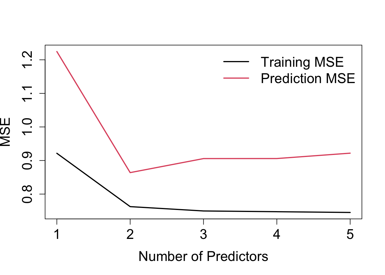

Figure 1.1: Training MSE and prediction MSE against number of predictors for the example discussed in the text.

Notice the following:

• Training error: steady (negligible) decline after adding $x_3$ – not really obvious how many predictors to include.
• Prediction error: clearly here one would select the model with $x_1$ and $x_2$!
• Prediction errors are larger than training errors – this is generally always the case!

1.1.4 R-squared

The R-squared value is another metric for evaluating model fit $$R^2 = 1 - \frac{RSS}{TSS},$$ where $TSS=\sum_{i=1}^{n} (y_i-\bar{y})^2$ is the Total Sum of Squares. As we know, $R^2$ ranges from 0 (worst fit) to 1 (perfect fit).

$R^2$ is just a function of $-RSS$ (since $TSS$ is a constant), so as we add further predictors $R^2$ will just increase.

In the case of $n=p$ we would have an $R^2$ value of 1 (overfitting).

In Figure 1.2, we show the value of $R^2$ against the number of predictors in the model for the example of Section 1.1.3.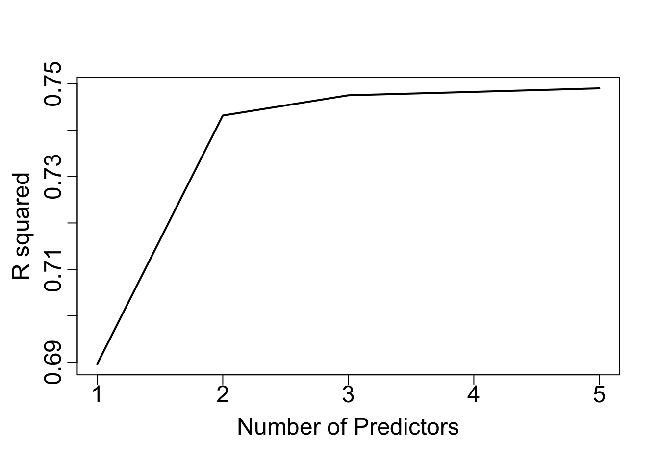

Figure 1.2: R-squared values against number of predictors for the example discussed in the text.

1.1.5 So, which model?

Given that in practice we may not wish to exclude part of the data for calculating a prediction error using validation (Section 1.1.2), we have two choices:

• directly estimate prediction error using cross-validation techniques (Section 1.1.6). This is computational by nature.
• indirectly estimate prediction error by making an adjustment to the training error that accounts for overfitting. Here, we have several model selection criteria available (Section 1.2).

We will proceed to look into these two options in the following sections.

1.1.6 Cross-Validation

k-fold Cross-validation (CV) involves randomly dividing the set of $n$ observations into $k$ groups (or folds) of approximately equal size.
Then, for each group $i=1,...,k$:

• Fold $i$ is treated as a validation set, and the model is fit on the remaining $k-1$ folds.
• The $MSE_i$ is then computed based on the observations of the held out fold $i$.

This process results in $k$ estimates of the test error $MSE_1,...,MSE_k$. The $k$-fold CV estimate is computed by averaging these values. $$CV_{(k)} = \frac{1}{k} \sum_{i=1}^{k} MSE_i$$

Figure 1.3 illustrates this nicely.

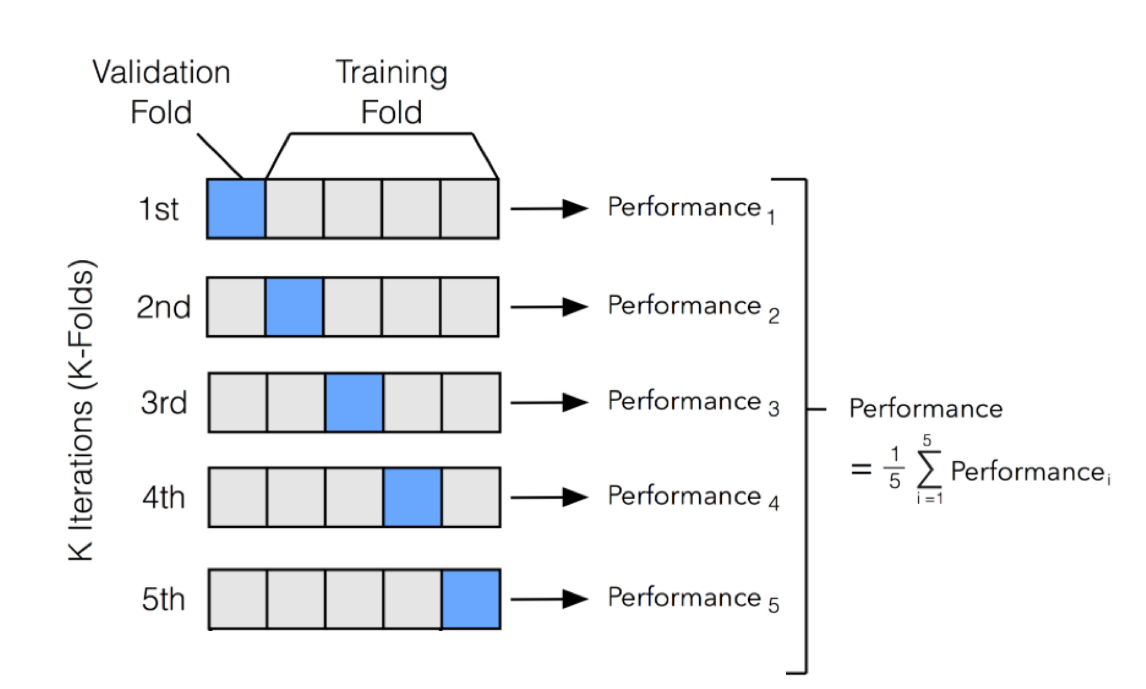
Figure 1.3: An illustration of k-fold CV with 5 folds.

1.2 Model Selection Criteria

As an alternative to the direct estimation of prediction error considered in Section 1.1.6, we now consider a number of indirect techniques that involve adjusting the training error for the model size. These approaches can be used to select among a set of models with different numbers of variables. We proceed to consider four such criteria.

1.2.1 $C_p$

For a given model with $d$ predictors (out of the available $p$ predictors) Mallows’ $C_p$ criterion is $$C_p = \frac{1}{n}(RSS + 2 d \hat{\sigma}^2),$$ where $RSS$ is the residual sum of squares for the model of interest (with $d$ predictors), and $\hat{\sigma}^2=RSS_p/(n-p-1)$ is an estimate of the error variance for the full model with all $p$ possible predictors included. As such, we use $RSS_p$ to denote the Residual Sum of Squares for the full model with all $p$ possible predictors included.

In practice, we choose the model which has the minimum $C_p$ value: so we essentially penalise models of higher dimensionality (the larger $d$ is the greater the penalty).

1.2.2 AIC

For linear models (with normal errors, as is often assumed), Mallows’ $C_p$ is equivalent to the Akaike Information Criterion (AIC) (as the two are proportional), this being given by $$AIC = \frac{1}{n\hat{\sigma}^2}(RSS + 2 d \hat{\sigma}^2).$$

1.2.3 BIC

Another metric is the Bayesian information criterion (BIC) $$BIC = \frac{1}{n\hat{\sigma}^2}(RSS + \log(n)d \hat{\sigma}^2),$$ where again the model with the minimum BIC value is selected

In comparison to $C_p$ or AIC, where the penalty is $2d \hat{\sigma}^2$, the BIC penalty is $\log(n)d \hat{\sigma}^2$. This means that generally BIC has a heavier penalty (because $\log(n)>2$ for $n>7$), thus BIC selects models with fewer variables than $C_p$ or AIC.

In general, all three criteria are based on rigorous theoretical asymptotic ($n\rightarrow \infty$) justifications.

1.2.4 Adjusted R-squared value

A simple method which is not backed up by statistical theory, but that often works well in practice, is to simply adjust the $R^2$ metric by taking into account the number of predictors.

The adjusted $R^2$ value for a model with $d$ variables is calculated as follows $$\mbox{Adjusted~} R^2 = 1 - \frac{RSS/(n-d-1)}{TSS/(n-1)}.$$
In this case we choose the model with the maximum adjusted $R^2$ value.

1.2.5 Example

By plotting the various model selection criteria against the number of predictors (Figure 1.4), we can see that, in our example, $C_p$, AIC and BIC are in agreement (2 predictors). Adjusted $R^2$ would select 3 predictors.

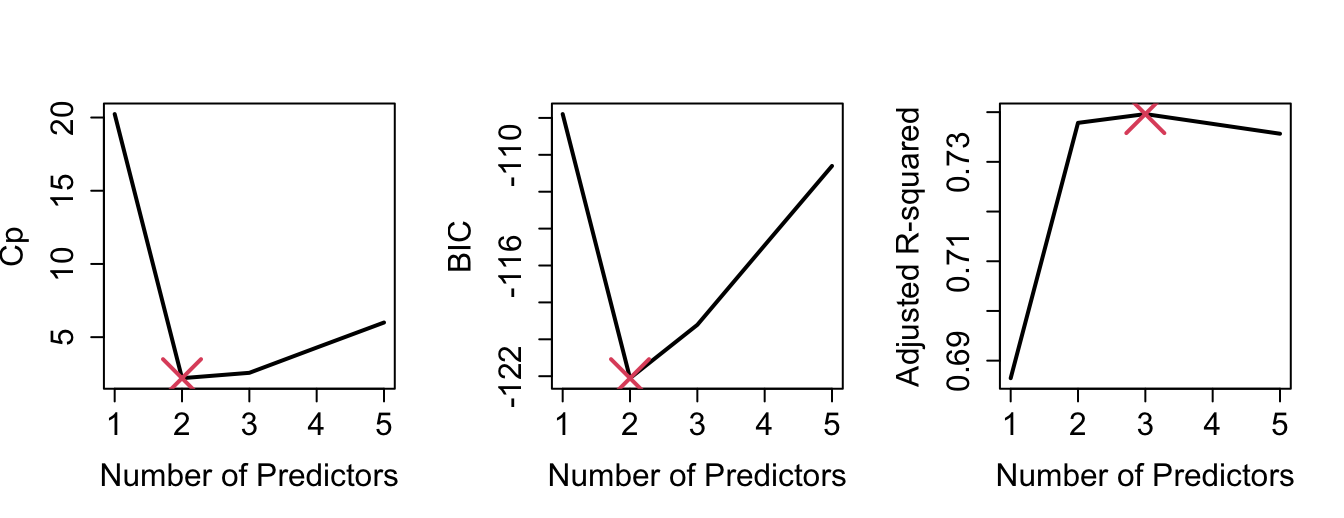
Figure 1.4: Various model selection criteria against number of predictors.

1.2.6 Further points

• A shortcoming of the previous approaches is that they are not applicable for models that have more variables than the size of the sample ($d>n$).
• Also, in the setting of penalised regression (which we will see later on in the course) deciding what $d$ actually is becomes a bit problematic.
• CV is an effective computational tool which can be used in all settings.

---

2. For the purposes of this illustration, we add the variables by index order, so three predictors corresponds to $x_1,x_2,x_3$ etc. How we should select $x_1$ and $x_2$ when we don’t know which variables are important comes later!↩︎