Chapter 5 Choosing \(\lambda\)
5.1 Importance of \(\lambda\)
- As we have seen, the penalty parameter \(\lambda\) is of crucial importance in penalised regression.
- For \(\lambda=0\) we essentially just get the LS estimates of the full model.
- For very large \(\lambda\): all ridge estimates become extremely small, while all lasso estimates are exactly zero!
We require a principled way to fine-tune \(\lambda\) in order to get optimal results.
5.2 Selection Criteria?
- In Chapter 1, we used the selection criteria \(C_p\), BIC and adjusted-\(R^2\) as criteria for choosing particular models during model search methods.
- Perhaps we can do that here, for instance, by defining a grid of values for \(\lambda\) and calculating the corresponding \(C_p\) under each model, before then finding the model with the corresponding \(\lambda\) that yields the lowest \(C_p\) value?
- Not really - the problem is that all these techniques depend on model dimensionality (number of predictors).
- With model-search methods we choose a model with \(d\) predictors, so it is clear that the model’s dimensionality is \(d\).
- Shrinkage methods, however, penalise dimensionality in a different way - the very notion of model dimensionality becomes obscure somehow - does a constrained predictor count towards dimensionality in the same way as an unconstrained one?
5.2.1 Example - Regularisation Paths
We now return to theCredit data example of Section 4.2.1, where we saw the standardised coefficient values against \(\lambda\) for each of the 10 possible predictors. Figure 5.16 shows a similar plot for lasso regression.
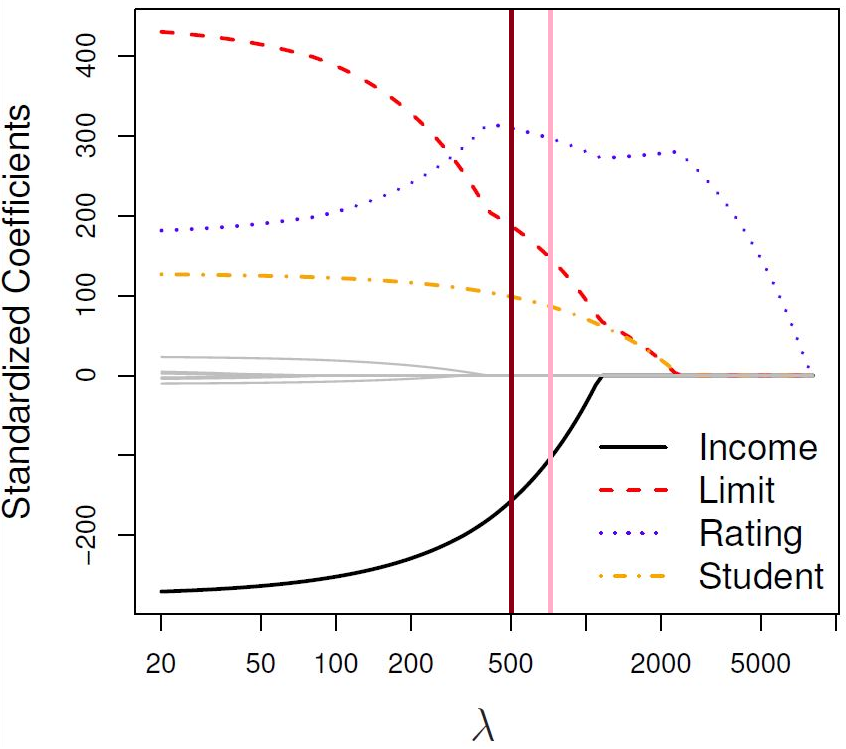
Figure 5.1: The standardised lasso regression coefficients for the Credit dataset, as a function of \(\lambda\).
The brown line highlights a specific model in the path. This model contains predictors Income, Limit, Rating and Student, so \(d=4\).
The pink line highlights another model which contains the same predictors.
So, in both models \(d=4\), but they are not the same model, because their regression coefficients are different! Again one should ask how the dimension penalty would even be applied in \(C_p\), for example - should the dimensionality penalty be the same for both of these models?
5.3 Cross-Validation
The only viable strategy is \(K\)-fold cross-validation. The steps are the following:
- Choose the number of folds \(K\).
- Split the data accordingly into training and testing sets.
- Define a grid of values for \(\lambda\).
- For each \(\lambda\) calculate the validation Mean Squared Error (MSE) within each fold.
- For each \(\lambda\) calculate the overall cross-validation MSE.
- Locate under which \(\lambda\) cross-validation MSE is minimised. This value of \(\lambda\) is known as the minimum_CV \(\lambda\).
Seems difficult, but fortunately glmnet in R will do all of these things for us automatically! We will explore using cross-validation for choosing \(\lambda\) further via practical demonstration.
5.4 Practical Demonstration
We will continue analysing the Hitters dataset included in package ISLR, this time applying the method of ridge regression.
5.4.1 Removing missing entries
We perform the usual steps of removing missing data, as seen in Section 2.4.
library(ISLR)
Hitters = na.omit(Hitters)
dim(Hitters)
## [1] 263 20sum(is.na(Hitters))## [1] 05.4.2 Ridge regression
In this part again we call the response y and extract the matrix of predictors, which we call x using the command model.matrix().
y = Hitters$Salary
x = model.matrix(Salary~., Hitters)[,-1] # Here we exclude the first column
                                         # because it corresponds to the
                                         # intercept term.
head(x)
## AtBat Hits HmRun Runs RBI Walks Years CAtBat CHits CHmRun CRuns CRBI
## -Alan Ashby 315 81 7 24 38 39 14 3449 835 69 321 414
## -Alvin Davis 479 130 18 66 72 76 3 1624 457 63 224 266
## -Andre Dawson 496 141 20 65 78 37 11 5628 1575 225 828 838
## -Andres Galarraga 321 87 10 39 42 30 2 396 101 12 48 46
## -Alfredo Griffin 594 169 4 74 51 35 11 4408 1133 19 501 336
## -Al Newman 185 37 1 23 8 21 2 214 42 1 30 9
## CWalks LeagueN DivisionW PutOuts Assists Errors NewLeagueN
## -Alan Ashby 375 1 1 632 43 10 1
## -Alvin Davis 263 0 1 880 82 14 0
## -Andre Dawson 354 1 0 200 11 3 1
## -Andres Galarraga 33 1 0 805 40 4 1
## -Alfredo Griffin 194 0 1 282 421 25 0
## -Al Newman 24 1 0 76 127 7 0For implementing cross-validation (CV) in order to select \(\lambda\) we will have to use the function cv.glmnet() from library glmnet. After loading library glmnet, we have a look at the help document by typing ?cv.glmnet. We see the argument nfolds = 10, so the default option is 10-fold CV (this is something we can change if we want to).
To perform cross-validation for selection of \(\lambda\) we simply run the following:
library(glmnet)

set.seed(1)
ridge.cv = cv.glmnet(x, y, alpha=0)
We extract the names of the output components as follows:
names( ridge.cv )## [1] "lambda" "cvm" "cvsd" "cvup" "cvlo" "nzero"
## [7] "call" "name" "glmnet.fit" "lambda.min" "lambda.1se" "index"lambda.min provides the optimal value of \(\lambda\) as suggested by the cross-validation MSEs.
ridge.cv$lambda.min## [1] 25.52821lambda.1se provides a different value of \(\lambda\), known as the 1-standard error (1-se) \(\lambda\). This is the maximum value that \(\lambda\) can take while still falling within the one standard error interval of the minimum_CV \(\lambda\).
ridge.cv$lambda.1se ## [1] 1843.343We see that in this case the 1-se \(\lambda\) is much larger than the min-CV \(\lambda\). This means that we expect the coefficients under 1-se \(\lambda\) to be much smaller. We can see that this is indeed the case by looking at the corresponding coefficients from the two models, rounding them to 3 decimal places.
round(cbind(
  coef(ridge.cv, s = 'lambda.min'),
  coef(ridge.cv, s = 'lambda.1se')),   # here we can also use coef(ridge.cv)
                                       # becauce 'lambda.1se' is the default
  digits = 3 )
## 20 x 2 sparse Matrix of class "dgCMatrix"
## s1 s1
## (Intercept) 81.127 159.797
## AtBat -0.682 0.102
## Hits 2.772 0.447
## HmRun -1.366 1.289
## Runs 1.015 0.703
## RBI 0.713 0.687
## Walks 3.379 0.926
## Years -9.067 2.715
## CAtBat -0.001 0.009
## CHits 0.136 0.034
## CHmRun 0.698 0.254
## CRuns 0.296 0.069
## CRBI 0.257 0.071
## CWalks -0.279 0.066
## LeagueN 53.213 5.396
## DivisionW -122.834 -29.097
## PutOuts 0.264 0.068
## Assists 0.170 0.009
## Errors -3.686 -0.236
## NewLeagueN -18.105 4.458Let’s plot the results based on the output of ridge.cv using plot. What is plotted is the estimated CV MSE for each value of (log) \(\lambda\) on the \(x\)-axis. The dotted line on the far left indicates the value of \(\lambda\) which minimises CV error. The dotted line roughly in the middle of the \(x\)-axis indicates the 1-standard-error \(\lambda\) - recall that this is the maximum value that \(\lambda\) can take while still falling within the on standard error interval of the minimum-CV \(\lambda\). The second line of code has manually added a dot-dash horizontal line at the upper end of the 1-standard deviation interval of the MSE at the minimum-CV \(\lambda\) to illustrate this point further.
plot(ridge.cv)
abline( h = ridge.cv$cvup[ridge.cv$index[1]], lty = 4 )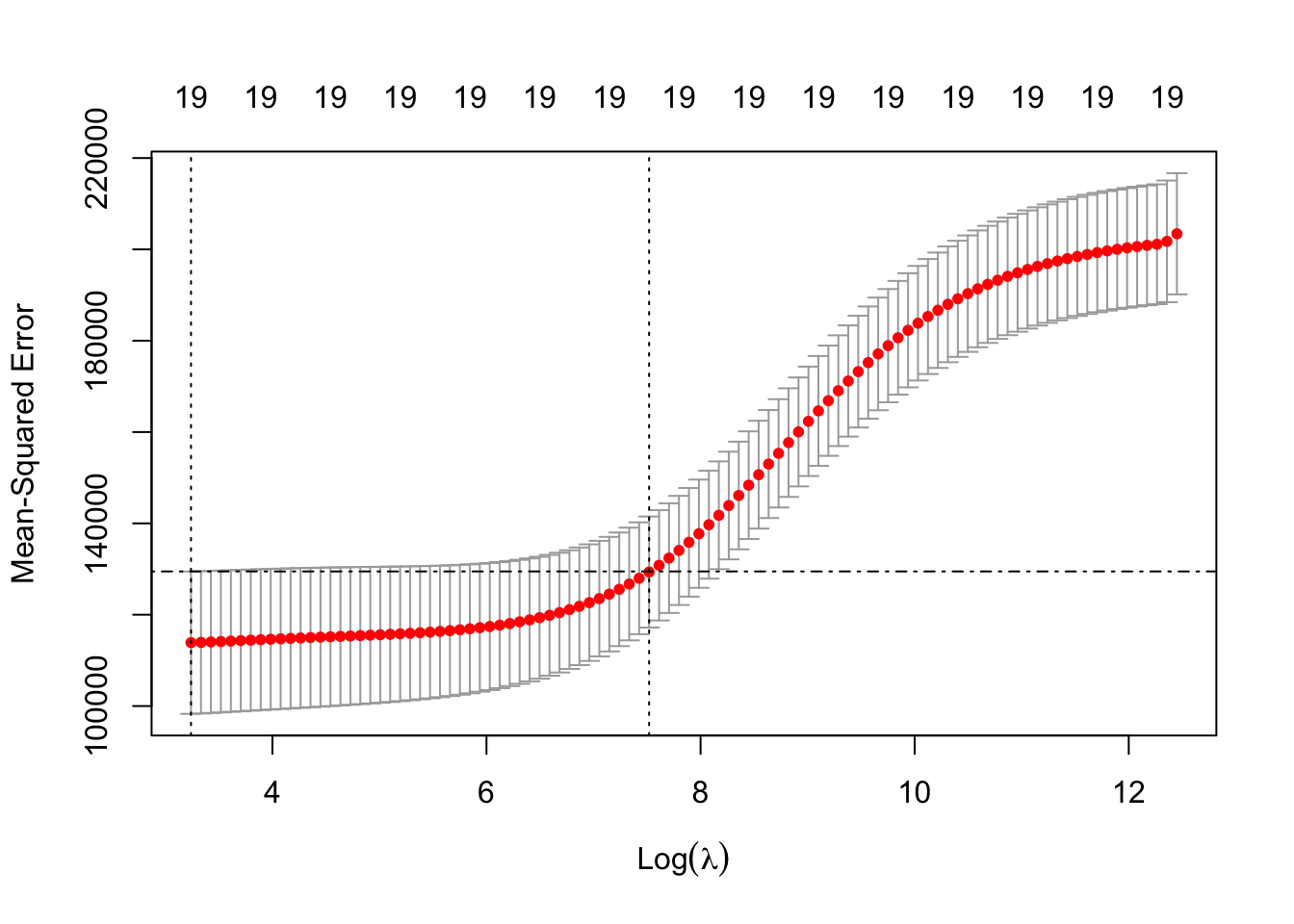
We can also plot the ridge regularisation paths and add the minimum-CV and 1-se \(\lambda\) values to the plot.
ridge = glmnet(x, y, alpha = 0)
plot(ridge, xvar = 'lambda')
abline(v = log(ridge.cv$lambda.min), lty = 3) # careful to use the log here
                                              # and below
abline(v = log(ridge.cv$lambda.1se), lty = 3)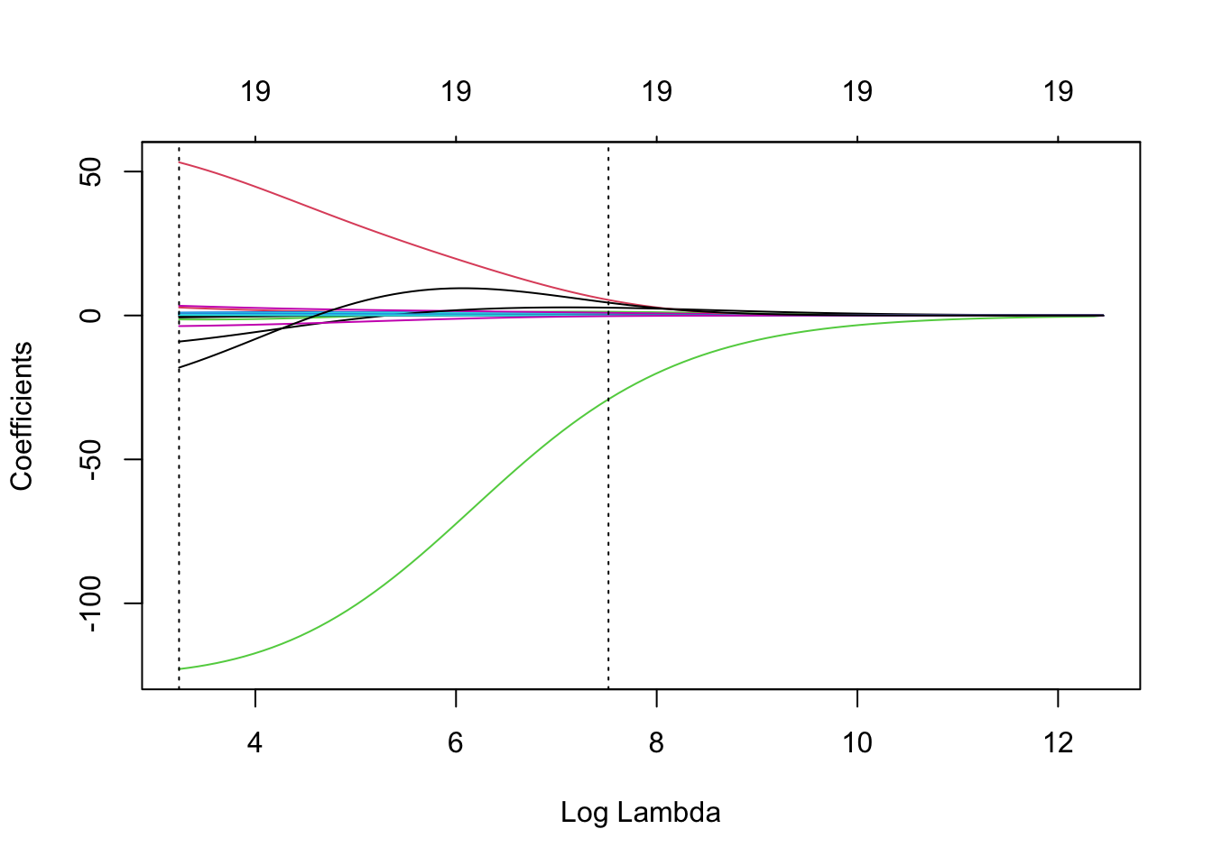
Important note: Any method/technique that relies on validation/cross-validation is subject to variability. If we re-run this code under a different random seed results will change.
5.4.3 Sparsifying the ridge coefficients?
One thing mentioned in Chapter 3 is that one can potentially consider some kind of post-hoc analysis in order to set some of the ridge coefficients equal to zero. A very simplistic approach is to just examine the ranking of the absolute coefficients and decide to use a “cutting-threshold”. We can use a combination of the commands sort() and abs() for this.
beta.1se =   coef( ridge.cv, s = 'lambda.1se' )[-1]
rank.coef = sort( abs( beta.1se ), decreasing = TRUE )
rank.coef
## [1] 29.096663826 5.396487460 4.457548079 2.714623469 1.289060569 0.925962429
## [7] 0.702915318 0.686866069 0.446840519 0.253594871 0.235989099 0.102483884
## [13] 0.071334608 0.068874010 0.067805863 0.066114944 0.034359576 0.009201998
## [19] 0.008746278The last two coefficients are quite small, so we could potentially set these two equal to zero (setting a threshold of say, 0.01). Equivalently we may set a larger threshold of say, 1, in which case we would remove far more variables from the model. We could check whether this sparsification would offer any benefits in terms of predictive performance by, for example, using K-fold cross-validation to evaluate the standard ridge regression fit (using glmnet with alpha = 0) with the \(i\)th fold excluded, and predicting the output for the \(i\)th fold using predict (see ?predict.glmnet for details).
5.4.4 Lasso regression
As we did with ridge, we can use the function cv.glmnet() to find the min-CV \(\lambda\) and the 1 standard error (1-se) \(\lambda\) under lasso. The code is the following.
set.seed(1)
lasso.cv = cv.glmnet(x, y)
lasso.cv$lambda.min
## [1] 1.843343lasso.cv$lambda.1se ## [1] 69.40069We see that in this case the 1-se \(\lambda\) is much larger than the min-CV \(\lambda\). This means that we expect the coefficients under 1-se \(\lambda\) to be much smaller (maybe exactly zero). Let’s have a look at the corresponding coefficients from the two models, rounding them to 3 decimal places.
round(cbind(
  coef(lasso.cv, s = 'lambda.min'),
  coef(lasso.cv, s = 'lambda.1se')),   # here we can also use coef(lasso.cv)
                                       # becauce 'lambda.1se' is the default
3)
## 20 x 2 sparse Matrix of class "dgCMatrix"
## s1 s1
## (Intercept) 142.878 127.957
## AtBat -1.793 .
## Hits 6.188 1.423
## HmRun 0.233 .
## Runs . .
## RBI . .
## Walks 5.148 1.582
## Years -10.393 .
## CAtBat -0.004 .
## CHits . .
## CHmRun 0.585 .
## CRuns 0.764 0.160
## CRBI 0.388 0.337
## CWalks -0.630 .
## LeagueN 34.227 .
## DivisionW -118.981 -8.062
## PutOuts 0.279 0.084
## Assists 0.224 .
## Errors -2.436 .
## NewLeagueN . .Finally, lets plot the results of the object lasso.cv which we have created, and compare them to that of the lasso object generated in Section 4.4.
par(mfrow=c(1,2))
plot(lasso.cv)
lasso = glmnet(x, y)
plot(lasso, xvar = 'lambda')
abline(v = log(lasso.cv$lambda.min), lty = 3) # careful to use the log here
                                              # and below
abline(v = log(lasso.cv$lambda.1se), lty = 3)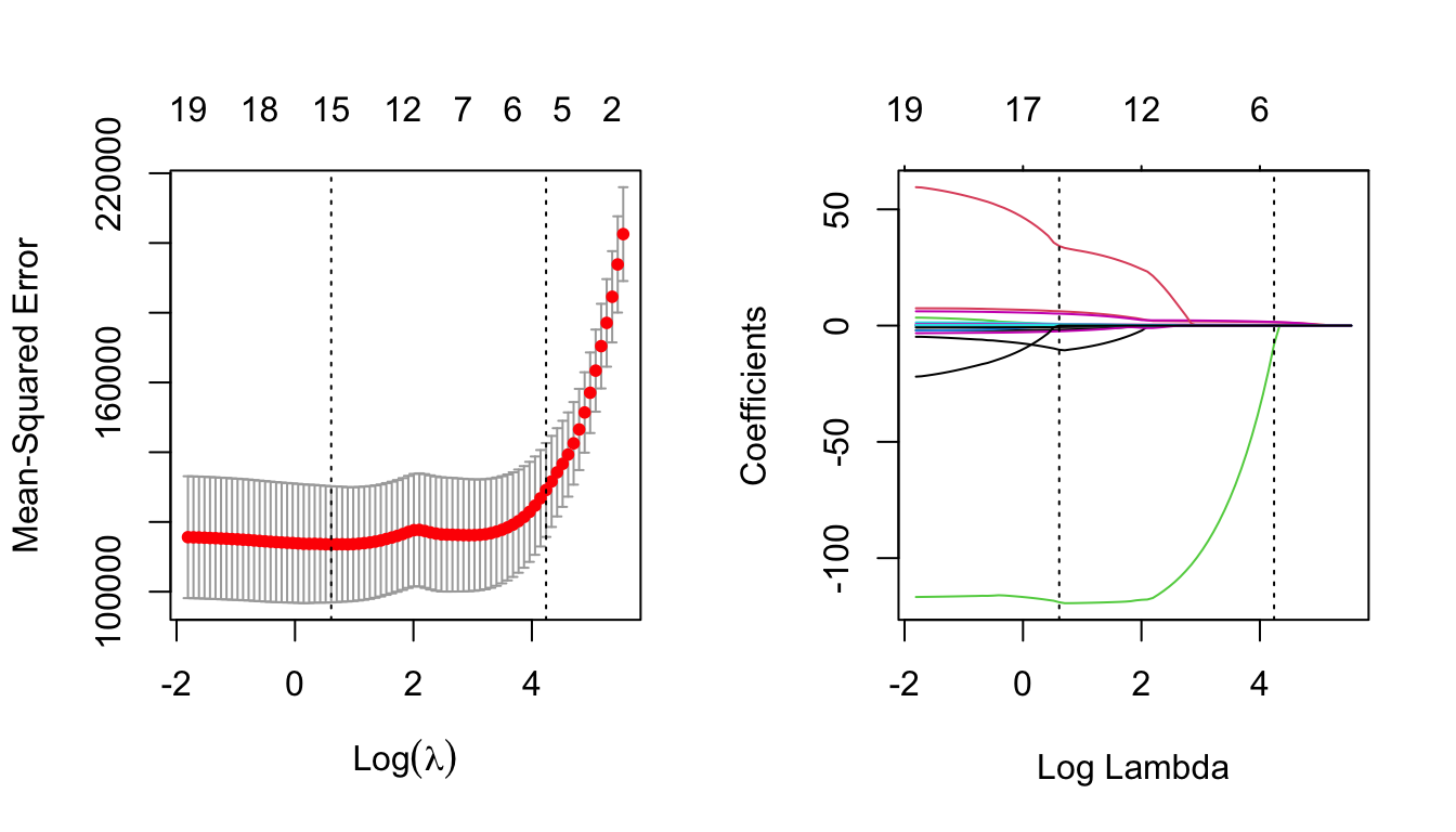
Notice now how the numbers across the top of the left-hand plot decrease as \(\lambda\) increases. This is indicating how many predictors are included for the corresponding \(\lambda\) value.
5.4.5 Comparing Predictive Performance for Different \(\lambda\)
We can investigate which of the two different \(\lambda\)-values (minimum-CV and 1-se) may be preferable in terms of predictive performance using the following code. Here, we split the data into a training and test set. We then use cross-validation to find minimum-CV \(\lambda\) and 1-se \(\lambda\), and use the resulting model to predict the response at the test data, comparing it to the actual response values by evaluating the correlation values between them. We then repeat this procedure many times using different splits in the data.
repetitions = 50
cor.1 = c()
cor.2 = c()

set.seed(1)
for(i in 1:repetitions){

  # Step (i) data splitting
  training.obs = sample(1:263,  175)
  y.train = Hitters$Salary[training.obs]
  x.train = model.matrix(Salary~., Hitters[training.obs, ])[,-1]
  y.test = Hitters$Salary[-training.obs]
  x.test = model.matrix(Salary~., Hitters[-training.obs, ])[,-1]

  # Step (ii) training phase
  lasso.train = cv.glmnet(x.train, y.train)

  # Step (iii) generating predictions
  predict.1 = predict(lasso.train, x.test, s = 'lambda.min')
  predict.2 = predict(lasso.train, x.test, s = 'lambda.1se')

  # Step (iv) evaluating predictive performance
  cor.1[i] = cor(y.test, predict.1)
  cor.2[i] = cor(y.test, predict.2)
}

boxplot(cor.1, cor.2, names = c('min-CV lasso','1-se lasso'),
        ylab = 'Test correlation', col = 7)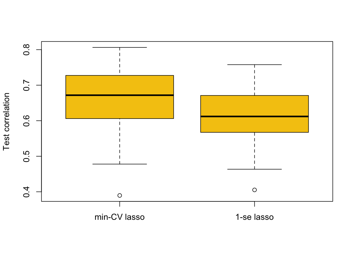
The approach based on min-CV is better, which makes sense as it minimised the cross-validation error (in cv.glmnet) in the first place. The 1-se \(\lambda\) can be of benefit in some cases for selecting models with fewer predictors that may be more interpretable. However, in applications where the 1-se \(\lambda\) is much larger than the min-CV \(\lambda\) (like here) we in general expect results as above.