Chapter 3 Ridge Regression
3.1 Introduction to Shrinkage
In Part I, we have seen discrete model search methods, where one option is to pick the best model based on information criteria (e.g. \(C_p,\) BIC, etc.). In this case we generally seek the minimum of
\[\underbrace{\mbox{model fit}}_{\mbox{RSS}}~ + ~{\mbox{penalty on model dimensionality}}\]
across models of differing dimensionality (number of predictors).
Shrinkage methods offer a continuous analogue (which is much faster). In this case we train only the full model, but the estimated regression coefficients minimise a general solution of the form \[\underbrace{\mbox{model fit}}_{\mbox{RSS}}~ + ~{\mbox{penalty on size of coefficients}}.\] This approach is called penalised or regularised regression.
3.2 Minimisation
Recall that Least Squares (LS) produces estimates of \(\beta_0,\, \beta_1,\, \beta_2,\, \ldots,\, \beta_p\) by minimising \[RSS = \sum_{i=1}^{n} \Bigg( y_i - \beta_0 - \sum_{j=1}^{p}\beta_j x_{ij}\Bigg)^2. \]
On the other hand, ridge regression minimises \[\underbrace{\sum_{i=1}^{n} \Bigg( y_i - \beta_0 - \sum_{j=1}^{p}\beta_j x_{ij}\Bigg)^2}_{\mbox{model fit}} + \underbrace{\lambda\sum_{j=1}^p\beta_j^2}_{\mbox{penalty}} = RSS + \lambda\sum_{j=1}^p\beta_j^2,\] where \(\lambda\ge 0\) is a tuning parameter. The role of this parameter is crucial; it controls the trade-off between model fit and the size of the coefficients. We will see later how we tune \(\lambda\)…
For now, observe that:
- when \(\lambda=0\) the penalty term has no effect and the ridge solution is the same as the LS solution.
- as \(\lambda\) gets larger, naturally the penalty term gets larger; so in order to minimise the entire function (model fit + penalty) the regression coefficients will necessarily get smaller!
- Unlike LS, ridge regression does not produce one set of coefficients, it produces different sets of coefficients for different values of \(\lambda\)!
- As \(\lambda\) is increasing the coefficients are shrunk towards 0 (for really large \(\lambda\) the coefficients are almost 0).
3.2.1 Example - Regularisation Paths
We here illustrate the effect of varying the tuning parameter \(\lambda\) on the ridge regression coefficients. We consider the Credit dataset in R (package ISLR). We do not worry about the code here - relevant coding for ridge regression will be covered in the practical demonstration of Section 3.6. You may, however, want to explore the help file for this dataset (remember to first install the ISLR library if you have not yet done so):
library("ISLR")
data(Credit)
?Credit
Importantly, we are here interested in predicting credit card Balance from the other variables, which are treated as predictors.
Income coefficient as \(\lambda\) is varied.
At the extreme left-hand side of the plot, \(\lambda\) is very close to zero and the coefficients for all predictors are relatively large (corresponding to the LS coefficients). As \(\lambda\) increases (from left to right along the \(x\)-axis), the ridge regression coefficient estimates shrink towards zero. When \(\lambda\) is extremely large, then all of the ridge coefficient estimates are basically zero (corresponding to the null model that contains no predictors). It should be noted that whilst the ridge coefficient estimates tend to decrease in general as \(\lambda\) increases, individual coefficients, such as Rating and Income in this case, may occasionally increase as \(\lambda\) increases.
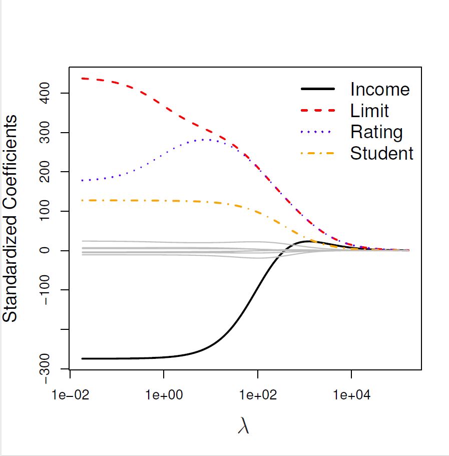
Figure 3.1: The standardised ridge regression coefficients for the Credit dataset, as a function of \(\lambda\).
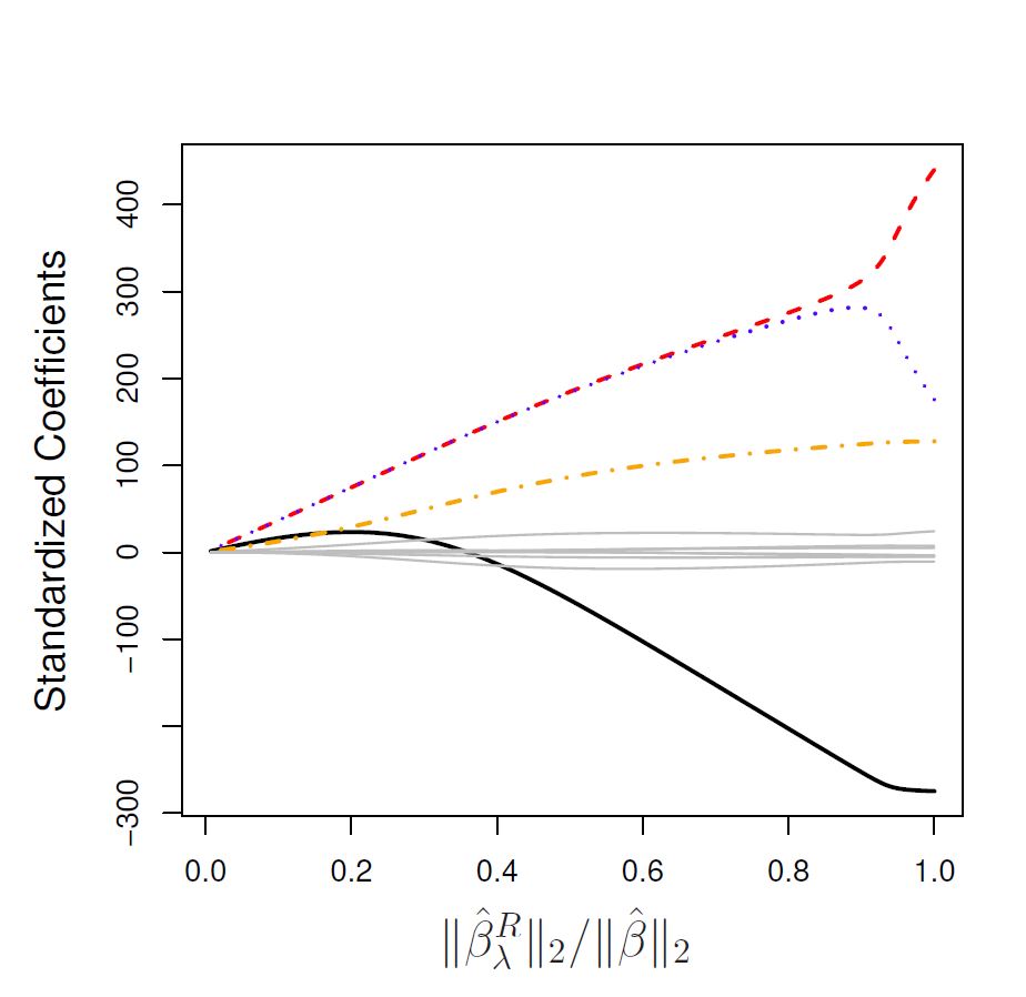
Figure 3.2: The standardised ridge regression coefficients for the Credit dataset, as a function of \(||\hat{\beta}_\lambda^R||_2/||\hat{\beta}||_2\).
3.3 Bias-Variance Trade-Off
For a carefully chosen \(\lambda\), ridge regression can significantly outperform LS in terms of estimation (and thus prediction). We discuss two cases when this is particularly true.
3.3.1 Multicollinearity
The first is in the presence of multicollinearity, which we explore via the following simulation study. This is a simulation study because we simulate data based on a known model, add some random noise, and then investigate how different methods use this data to estimate the regression parameters. We can then evaluate the performance of the method based on how close the estimated parameter values are to the true values.
We assume a correct model of \[y=x_1-x_2+\epsilon\] so that we have true generating \(\beta_0=0\), \(\beta_1=1\) and \(\beta_2 = -1\), and noise term \(\epsilon\sim\mathcal{N}(0,1)\). In other words, for any specified \((x_1,x_2)\), we evaluate the response \(x_1-x_2\) before adding random noise.
Rather than sampling the training data independently, however, we assume a high level of collinearity between \(x_1\) and \(x_2\) by simulating \(x_1\sim\mathcal{N}(0,1)\) and \(x_2\sim\mathcal{N}(0.9x_1,0.2^2)\). In other words, \(x_2\) is a scaling of \(x_1\) with just a small amount of random noise added - there is definitely correlation between the values of those predictors!
Feel free to look through the following code to understand how the simulation study is working and the plots below generated! Note that \((X^TX)^{-1}X^TY\) and \((X^TX + \lambda I)^{-1}X^TY\) are the regression coefficient estimates for LS and ridge respectively.
# Number of iterations for simulation study.
iter <- 50

# Number of training points.
n <- 10

# lambda coefficient - feel free to explore this parameter!
lambda <- 0.3

# Empty matrix of NAs for the regression coefficients, one for LS
# and one for ridge.
b_LS <- matrix( NA, nrow = 2, ncol = iter )
b_ridge <- matrix( NA, nrow = 2, ncol = iter )

# For each iteration...
for( i in 1:iter ){

  # As we can see x2 is highly correlated with x1 - COLLINEARITY!
  x1 <- rnorm( n )
  x2 <- 0.9 * x1 + rnorm( n, 0, 0.2 )

  # Design matrix.
  x <- cbind( x1, x2 )

  # y = x1 - x2 + e, where error e is N(0,1)
  y <- x1 - x2 + rnorm( n )

  # LS regression components - the below calculation obtains them given the
  # training data and response generated in this iteration, and stores
  # those estimates in the relevant column of the matrix b_LS.
  b_LS[,i]<- solve( t(x) %*% x ) %*% t(x) %*% y

  # Ridge regression components - notice that the only difference relative
  # to the LS estimates above is the addition of a lambda x identity matrix
  # inside the inverse operator.
  b_ridge[,i]<- solve( t(x) %*% x + lambda * diag(2) ) %*% t(x) %*% y

}

# Now we plot the results.  First, split the plotting window
# such that it has 1 row and 2 columns.
par(mfrow=c(1,2))

# Plot the LS estimates for beta_1.
plot( b_LS[1,], col = 'blue', pch = 16, ylim = c( min(b_LS), max(b_LS) ),
      ylab = 'Estimated coefficients', xlab = 'Least squares', bty ='l' )
# Add the LS estimates for beta_2 in a different colour.
points( b_LS[2,], col = 'red', pch = 17 )
# Add horizontal lines representing the true values of beta_1 and beta_2.
abline( a = 1, b = 0, col = 'blue' ) # Plot the true value of beta_1 = 1.
abline( a = -1, b = 0, col='red' ) # Plot the true value of beta_2 = -1.

# Do the same for the ridge estimates.
plot( b_ridge[1,], col = 'blue', pch = 16, ylim = c(min(b_LS), max(b_LS)),
      ylab = 'Estimated coefficients', xlab = 'Ridge', bty ='l' )
points( b_ridge[2,], col = 'red', pch = 17 )
abline( a = 1, b = 0, col = 'blue' )
abline( a = -1, b = 0, col = 'red' )

# Add a legend to this plot.
legend( 'bottomleft', cex = 1.3, text.col=c('blue','red'),
        legend = c( expression( beta[1] ),expression( beta[2] ) ),
        bty = 'n' )

# Add a title over the top of both plots.
mtext( expression( 'High correlations with'~n == 10~','~ p == 2 ),
       side = 3, line = -3, outer = TRUE )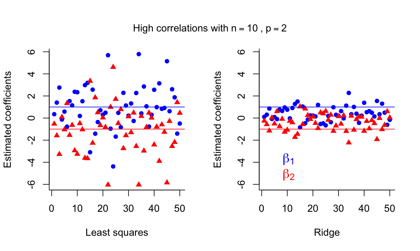
We can see that the LS coefficients are unbiased but are very unstable (high variance) in the presence of multicollinearity. This affects prediction error. Ridge regression introduces some bias but decreases the variance, which results in better predictions.
3.3.2 When \(p\) is close to \(n\)
The second case is when \(p\) is close to \(n\). We investigate this case by running the simulation above again, but this time sampling both \(x_1\) and \(x_2\) from a standard normal distribution \(\mathcal{N}(0,1)\) (making the two predictors independent) and lowering the number of training points to 3. I have removed the detailed comments this time - try to see (and understand!) how it is different to the simulation above.
iter <- 50
n <- 3
lambda <- 0.3

b_LS <- matrix( NA, nrow = 2, ncol = iter )
b_ridge <- matrix( NA, nrow = 2, ncol = iter )

for( i in 1:iter ){
  x1 <- rnorm( n )
  x2 <- rnorm( n )
  x <- cbind( x1, x2 )
  y <- x1 - x2 + rnorm( n )
  b_LS[,i]<- solve( t(x) %*% x ) %*% t(x) %*% y
  b_ridge[,i]<- solve( t(x) %*% x + lambda * diag(2) ) %*% t(x) %*% y
}

par(mfrow=c(1,2))
plot( b_LS[1,], col = 'blue', pch = 16, ylim = c( min(b_LS), max(b_LS) ),
      ylab = 'Estimated coefficients', xlab = 'Least squares', bty ='l' )
points( b_LS[2,], col = 'red', pch = 17 )
abline( a = 1, b = 0, col = 'blue' )
abline( a = -1, b = 0, col='red' )

plot( b_ridge[1,], col = 'blue', pch = 16, ylim = c(min(b_LS), max(b_LS)),
      ylab = 'Estimated coefficients', xlab = 'Ridge', bty ='l' )
points( b_ridge[2,], col = 'red', pch = 17 )
abline( a = 1, b = 0, col = 'blue' )
abline( a = -1, b = 0, col = 'red' )

# Add a legend to this plot.
legend( 'bottomleft', cex = 1.3, text.col=c('blue','red'),
        legend = c( expression( beta[1] ),expression( beta[2] ) ), bty = 'n' )

mtext( expression('No correlations with'~n == 3~','~ p == 2),
       side = 3, line = -3, outer = TRUE )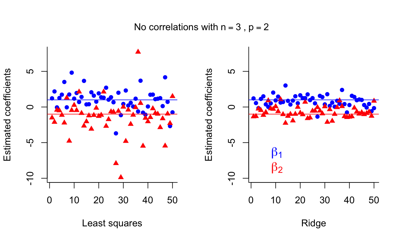
LS estimates suffer again from high variance. Ridge estimates are again more stable. Of course, having only \(n=3\) training runs isn’t ideal in any situation, but it illustrates how ridge estimates can be an improvement over LS.
You may want to run the simulation above again but increase the number of training points to compare how LS and ridge compare in a setting you may be more familiar with (that is, with reasonable \(n > p\) and without collinearity).
Many modern machine learning applications suffer from both these problems we have just explored - that is, \(p\) can be large (and of similar magnitude to \(n\)) and it is very likely that there will be strong correlations among the many predictors!
3.3.3 Bias-Variance Trade Off in Prediction Error
We illustrate the bias-variance trade-off nicely by varying the \(\lambda\) of ridge regression for a simulated dataset containing \(p=45\) predictors and \(n=50\) observations. We won’t worry about the details, but in this situation, we can see that the green curve, representing variance, initially decreases fast as \(\lambda\) increases. In contrast, the black curve, representing squared bias, initially increases only at a slow rate. This leads to the optimal \(\lambda\) in terms of Mean Squared Error being able to strike a good balance between variance and bias.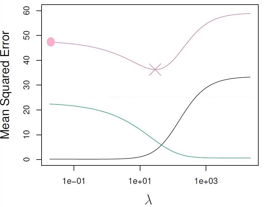
Figure 3.3: Squared bias (black), variance (green), and test mean squared error (pink) for the ridge regression predictions on a simulated dataset.
3.4 Scalability and Feature Selection
- Ridge is applicable for any number of predictors even when \(n < p\) - remember that LS solutions do not exist in this case. It is also much faster than the model-search based methods since we train only one model.
- Strictly speaking, ridge does not perform feature selection (since the coefficients are almost never exactly 0), but it can give us a good idea of which predictors are not influential and can be combined with post-hoc analysis based on ranking the absolute values of the coefficients.
3.5 Scaling
- The LS estimates are scale invariant: multiplying a feature \(X_j\) by some constant \(c\) will scale down \(\hat{\beta}_j\) by \(1/c\), so \(X_j\hat{\beta}_j\) will remain unaffected.
- In ridge regression (and any shrinkage method) the scaling of the features matters! If a relevant feature is in a smaller scale (that is, the numbers are smaller, e.g. using metres as opposed to millimetres) in relation to other features it will have a larger coefficient which constitutes a greater proportion of the penalty term and will thus shrink proportionally faster to zero.
- So, we want the features to be on the same scale.
- In practice, we standardise: \[ \tilde{x}_{ij} = \frac{x_{ij}}{\sqrt{\frac{1}{n} (x_{ij}-\bar{x}_j)^2}},\] so that all predictors have variance equal to one.
3.6 Practical Demonstration
We will continue analysing the Hitters dataset included in package ISLR, this time applying the method of ridge regression.
3.6.1 Removing missing entries
We perform the usual steps of removing missing data, as seen in Section 2.4.
library(ISLR)
Hitters = na.omit(Hitters)
dim(Hitters)
## [1] 263 20sum(is.na(Hitters))## [1] 03.6.2 Ridge regression
The first thing to do is to load up the package glmnet (remember to run the command install.packages('glmnet') the first time).
library(glmnet)## Loading required package: Matrix## Loaded glmnet 4.1-6Initially, we will make use of function glmnet() which implements ridge regression without cross-validation, but it does give a range of solutions over a grid of \(\lambda\) values. The grid is produced automatically - we do not need to specify anything. Of course, if we want to we can define the grid manually. Let’s have a look first at the help document of glmnet().
?glmnetA first important thing to observe is that glmnet() requires a different syntax than regsubsets() for declaring the response variable and the predictors. Now the response should be a vector and the predictor variables must be stacked column-wise as a matrix. This is easy to do for the response. For the predictors we have to make use of the model.matrix() command. Let us define as y the response and as x the matrix of predictors.
y = Hitters$Salary
x = model.matrix(Salary~., Hitters)[,-1] # Here we exclude the first column
                                         # because it corresponds to the
                                         # intercept.
head(x)
## AtBat Hits HmRun Runs RBI Walks Years CAtBat CHits CHmRun CRuns CRBI
## -Alan Ashby 315 81 7 24 38 39 14 3449 835 69 321 414
## -Alvin Davis 479 130 18 66 72 76 3 1624 457 63 224 266
## -Andre Dawson 496 141 20 65 78 37 11 5628 1575 225 828 838
## -Andres Galarraga 321 87 10 39 42 30 2 396 101 12 48 46
## -Alfredo Griffin 594 169 4 74 51 35 11 4408 1133 19 501 336
## -Al Newman 185 37 1 23 8 21 2 214 42 1 30 9
## CWalks LeagueN DivisionW PutOuts Assists Errors NewLeagueN
## -Alan Ashby 375 1 1 632 43 10 1
## -Alvin Davis 263 0 1 880 82 14 0
## -Andre Dawson 354 1 0 200 11 3 1
## -Andres Galarraga 33 1 0 805 40 4 1
## -Alfredo Griffin 194 0 1 282 421 25 0
## -Al Newman 24 1 0 76 127 7 0See how the command model.matrix() automatically transformed the categorical variables in Hitters with names League, Division and NewLeague to dummy variables with names LeagueN, DivisionW and NewLeagueN.
Other important things that we see in the help document are that glmnet() uses a grid of 100 values for \(\lambda\) (nlambda = 100) and that parameter alpha is used to select between ridge implementation and lasso implementation. The default option is alpha = 1 which runs lasso (see Chapter 4) - for ridge we have to set alpha = 0. Finally we see the default option standardize = TRUE, which means we do not need to standardize the predictor variables manually.
Now we are ready to run our first ridge regression!
ridge = glmnet(x, y, alpha = 0)Using the command names() we can find what is returned by the function. The most important components are "beta" and "lambda". We can easily extract each using the $ symbol.
names(ridge)## [1] "a0" "beta" "df" "dim" "lambda" "dev.ratio" "nulldev"
## [8] "npasses" "jerr" "offset" "call" "nobs"ridge$lambda## [1] 255282.09651 232603.53864 211939.68135 193111.54419 175956.04684 160324.59659
## [7] 146081.80131 133104.29670 121279.67783 110505.52551 100688.51919 91743.62866
## [13] 83593.37754 76167.17227 69400.69061 63235.32454 57617.67259 52499.07736
## [19] 47835.20402 43585.65633 39713.62675 36185.57761 32970.95062 30041.90224
## [25] 27373.06245 24941.31502 22725.59734 20706.71790 18867.19015 17191.08098
## [31] 15663.87273 14272.33745 13004.42232 11849.14529 10796.49988 9837.36858
## [37] 8963.44387 8167.15622 7441.60857 6780.51658 6178.15417 5629.30398
## [43] 5129.21213 4673.54706 4258.36202 3880.06088 3535.36696 3221.29471
## [49] 2935.12376 2674.37546 2436.79131 2220.31349 2023.06696 1843.34326
## [55] 1679.58573 1530.37596 1394.42158 1270.54501 1157.67329 1054.82879
## [61] 961.12071 875.73739 797.93930 727.05257 662.46322 603.61181
## [67] 549.98860 501.12913 456.61020 416.04621 379.08581 345.40887
## [73] 314.72370 286.76451 261.28915 238.07694 216.92684 197.65566
## [79] 180.09647 164.09720 149.51926 136.23638 124.13351 113.10583
## [85] 103.05782 93.90245 85.56042 77.95946 71.03376 64.72332
## [91] 58.97348 53.73443 48.96082 44.61127 40.64813 37.03706
## [97] 33.74679 30.74882 28.01718 25.52821dim(ridge$beta)## [1] 19 100ridge$beta[,1:3]## 19 x 3 sparse Matrix of class "dgCMatrix"
## s0 s1 s2
## AtBat 1.221172e-36 0.0023084432 0.0025301407
## Hits 4.429736e-36 0.0083864077 0.0091931957
## HmRun 1.784944e-35 0.0336900933 0.0369201974
## Runs 7.491019e-36 0.0141728323 0.0155353349
## RBI 7.912870e-36 0.0149583386 0.0163950163
## Walks 9.312961e-36 0.0176281785 0.0193237654
## Years 3.808598e-35 0.0718368521 0.0787191800
## CAtBat 1.048494e-37 0.0001980310 0.0002170325
## CHits 3.858759e-37 0.0007292122 0.0007992257
## CHmRun 2.910036e-36 0.0054982153 0.0060260057
## CRuns 7.741531e-37 0.0014629668 0.0016034328
## CRBI 7.989430e-37 0.0015098418 0.0016548119
## CWalks 8.452752e-37 0.0015957724 0.0017488195
## LeagueN -1.301217e-35 -0.0230232091 -0.0250669217
## DivisionW -1.751460e-34 -0.3339842326 -0.3663713386
## PutOuts 4.891197e-37 0.0009299203 0.0010198028
## Assists 7.989093e-38 0.0001517222 0.0001663687
## Errors -3.725027e-37 -0.0007293365 -0.0008021006
## NewLeagueN -2.585026e-36 -0.0036169801 -0.0038293583As we see above glmnet() defines the grid starting with large values of \(\lambda\). This is because this helps speeding up the optimisation procedure. Also, glmnet() performs some internal checks on the predictor variables in order to define the grid values. Therefore, it is generally better to let glmnet() define the grid automatically, rather than manually defining a grid. We further see that as expected ridge$beta had 19 rows (number of predictors) and 100 columns (length of the grid). Above the first 3 columns are displayed. Notice that ridge$beta does not return the estimates of the intercepts. We can use the command coef() for this, which returns all betas.
coef(ridge)[,1:3]## 20 x 3 sparse Matrix of class "dgCMatrix"
## s0 s1 s2
## (Intercept) 5.359259e+02 5.279266e+02 5.271582e+02
## AtBat 1.221172e-36 2.308443e-03 2.530141e-03
## Hits 4.429736e-36 8.386408e-03 9.193196e-03
## HmRun 1.784944e-35 3.369009e-02 3.692020e-02
## Runs 7.491019e-36 1.417283e-02 1.553533e-02
## RBI 7.912870e-36 1.495834e-02 1.639502e-02
## Walks 9.312961e-36 1.762818e-02 1.932377e-02
## Years 3.808598e-35 7.183685e-02 7.871918e-02
## CAtBat 1.048494e-37 1.980310e-04 2.170325e-04
## CHits 3.858759e-37 7.292122e-04 7.992257e-04
## CHmRun 2.910036e-36 5.498215e-03 6.026006e-03
## CRuns 7.741531e-37 1.462967e-03 1.603433e-03
## CRBI 7.989430e-37 1.509842e-03 1.654812e-03
## CWalks 8.452752e-37 1.595772e-03 1.748819e-03
## LeagueN -1.301217e-35 -2.302321e-02 -2.506692e-02
## DivisionW -1.751460e-34 -3.339842e-01 -3.663713e-01
## PutOuts 4.891197e-37 9.299203e-04 1.019803e-03
## Assists 7.989093e-38 1.517222e-04 1.663687e-04
## Errors -3.725027e-37 -7.293365e-04 -8.021006e-04
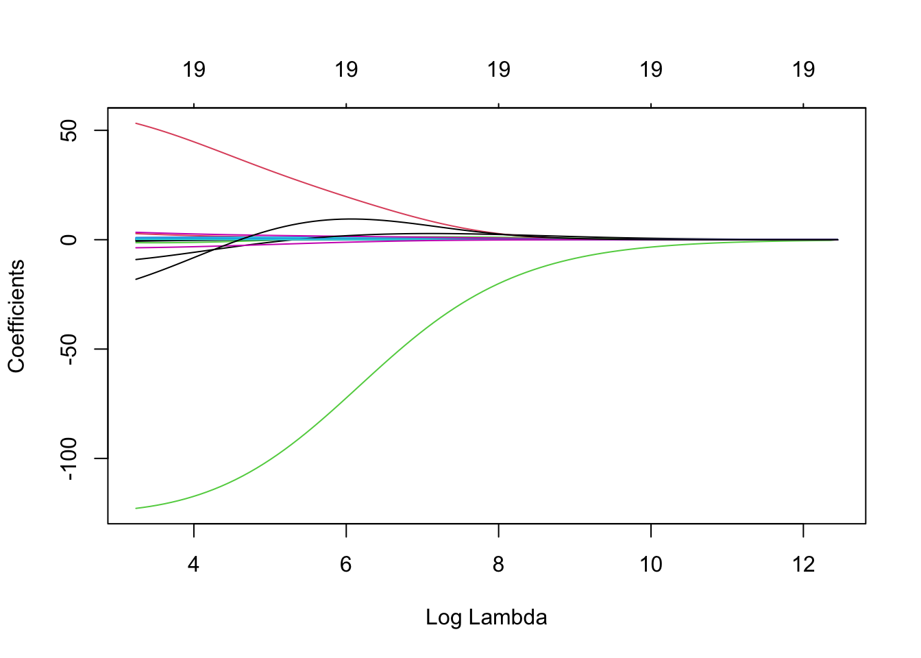
## NewLeagueN -2.585026e-36 -3.616980e-03 -3.829358e-03We can produce a plot similar to the ones seen previously via the following simple code. On the left we have the regularisation paths based on \(\log\lambda\). Specifying xvar is important, as the default is to plot the \(\ell_1\)-norm on the \(x\)-axis (see Chapter 4). Don’t worry about the row of 19’s along the top of the plot for now, except to note that this is the number of predictor variables. The reason for their presence will become clear in Chapter 4.
plot(ridge, xvar = 'lambda')