Chapter 4 The Lasso

4.1 Disadvantage of Ridge Regression

Unlike model search methods which select models that include subsets of predictors, ridge regression will include all $p$ predictors.
Recall in Figure 3.1 that the grey lines are the coefficient paths of irrelevant variables: always close to zero but never set exactly equal to zero!
We could perform a post-hoc analysis (see Section 5.4.3), but ideally we would like a method that sets these coefficients equal to zero automatically.

4.2 Lasso Regression

First of all: different ways to pronounce it - pick your favourite!
Lasso is a more recent shrinkage method.
Similar to ridge regression it penalises the size of the coefficients, but instead of the squares it penalises the absolute values.
The lasso regression estimates minimise the quantity \[{\sum_{i=1}^{n} \Bigg( y_i - \beta_0 - \sum_{j=1}^{p}\beta_j x_{ij}\Bigg)^2} + {\lambda\sum_{j=1}^p|\beta_j|} = RSS + \lambda\sum_{j=1}^p|\beta_j|\]
The only difference is that the $\beta_j^2$ term in the ridge regression penalty has been replaced by $|\beta_j|$ in the lasso penalty.
We say that the lasso uses an $\ell_1$ penalty as opposed to an $\ell_2$ penalty.
The $\ell_1$ norm of a coefficient vector $\beta$ is given by \[||\beta||_1 = \sum_{j=1}^p |\beta_j|\]
Lasso offers the same benefits as ridge:
- it introduces some bias but decreases the variance, so it improves predictive performance.
- it is extrememly scalable and can cope with $n<p$ problems.

As with ridge regression, the lasso shrinks the coefficient estimates towards zero. However, in the case of the lasso, the $\ell_1$ penalty has the effect of forcing some of the coefficient estimates to be exactly equal to zero when the tuning parameter $\lambda$ is sufficiently large. Hence, much like best subset selection, the lasso performs variable selection. As a result, models generated form the lasso are generally much easier to interpret than those produced by ridge regression. We say that the lasso yields sparse models, that is, models that involve only a subset of the variables. As with ridge regression, the choice of $\lambda$ is critical, but we defer discussion of this until Chapter 5.

4.2.1 Example - Regularisation Paths

We illustrate the effect of varying the tuning parameter $\lambda$ on the lasso coefficients using the Credit data example, as we did in Section 3.2.1 for ridge regression.

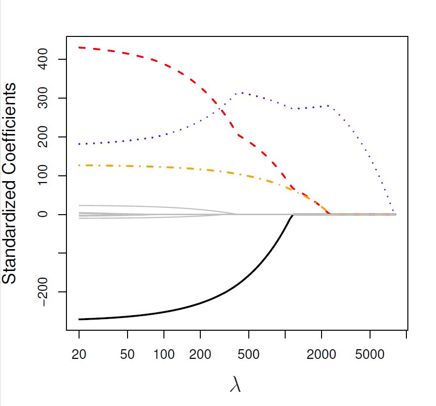
We can see from Figure 4.1 ⁵ that when $\lambda = 0$, the lasso simply gives the least squares fit. As $\lambda$ increases, the coefficient values in general decrease, however, each coefficient hits zero at some point for sufficiently large $\lambda$. As for ridge regression, individual coefficients can again occasionally increase as $\lambda$ increases.

$The standardised lasso regression coefficients for the `Credit` dataset, as a function of $\lambda$.$

Figure 4.1: The standardised lasso regression coefficients for the Credit dataset, as a function of $\lambda$.

We can also plot (Figure 4.2) the standardised coefficients as functions of $||\hat{\beta}_\lambda^L||_1/||\hat{\beta}||_1$, where $\hat{\beta}_\lambda^L$ is the vector of lasso regression coefficients. Moving from left to right, we can see that at first the lasso results in a model that contains only the Rating predictor. Then Student and Limit enter the model almost simultaneously, shortly followed by Income. Eventually, the remaining variables also enter the model. Hence, depending on the value of $\lambda$, the lasso can produce a model involving any number of predictors.

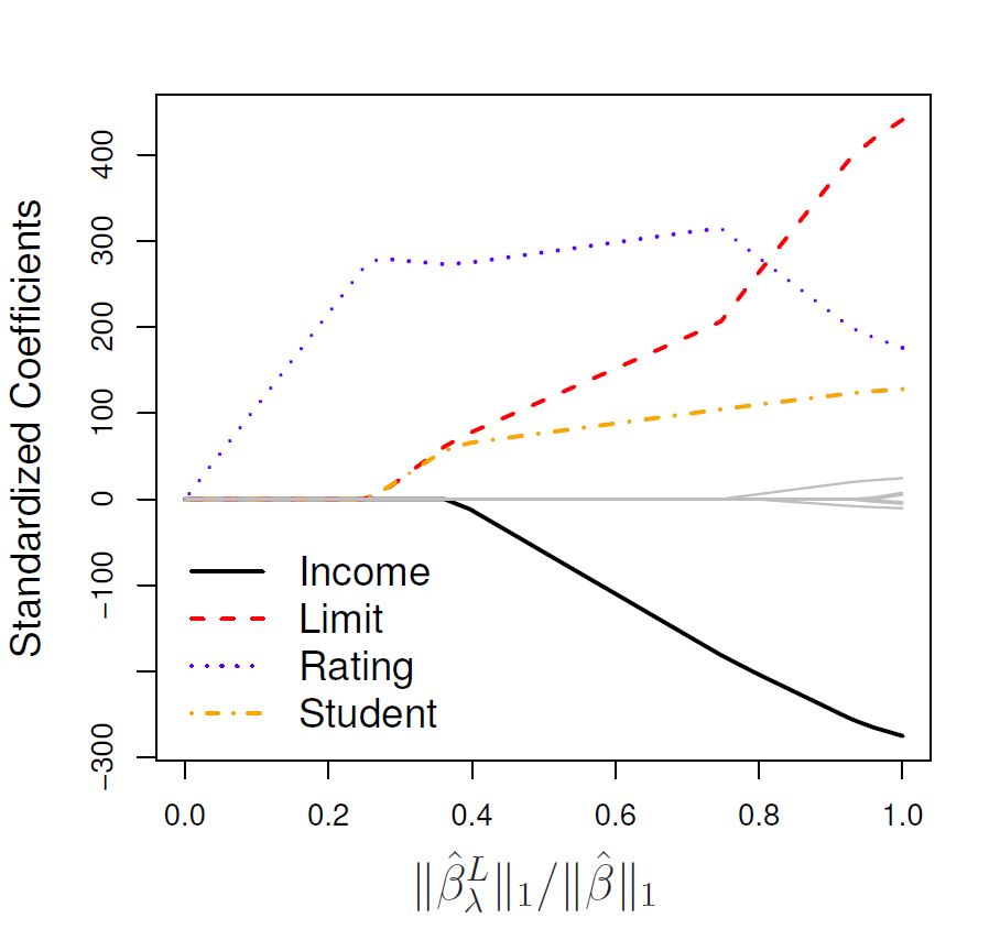
$The standardised lasso regression coefficients for the `Credit` dataset, as a function of $||\hat{\beta}_\lambda^L||_1/||\hat{\beta}||_1$.$

Figure 4.2: The standardised lasso regression coefficients for the Credit dataset, as a function of $||\hat{\beta}_\lambda^L||_1/||\hat{\beta}||_1$.

4.3 Ridge vs. Lasso

Here we make some comparisons between ridge regression and lasso regression.

4.3.1 Ridge and Lasso with $\ell$-norms

We have talked a little bit about the $\ell$-norms, but here we clarify the difference between ridge and lasso using them.

Lets just denote $\beta=(\beta_1,\ldots,\beta_p)$. Then a more compact representation of ridge and lasso minimisation is the following:

Ridge: ${\sum_{i=1}^{n} \Bigg( y_i - \beta_0 - \sum_{j=1}^{p}\beta_j x_{ij}\Bigg)^2} + {\lambda\Vert\beta\Vert_2^2}$, where $\Vert\beta\Vert_2=\sqrt{\beta_1^2 + \ldots + \beta_p^2}$ is the $\ell_2$-norm of $\beta$.
Lasso: ${\sum_{i=1}^{n} \Bigg( y_i - \beta_0 - \sum_{j=1}^{p}\beta_j x_{ij}\Bigg)^2} + {\lambda\Vert\beta\Vert_1}$, where $\Vert\beta\Vert_1={|\beta_1| + \ldots + |\beta_p|}$ is the $\ell_1$-norm of $\beta$.

That is why we say that ridge uses $\ell_2$-penalisation, while lasso uses $\ell_1$-penalisation.

4.3.2 Ridge and Lasso as Constrained Optimisation Problems

Ridge: minimise $\sum_{i=1}^{n} \Bigg( y_i - \beta_0 - \sum_{j=1}^{p}\beta_j x_{ij}\Bigg)^2$ subject to $\sum_{j=1}^p\beta_j^2 \le t$.
Lasso: minimise $\sum_{i=1}^{n} \Bigg( y_i - \beta_0 - \sum_{j=1}^{p}\beta_j x_{ij}\Bigg)^2$ subject to $\sum_{j=1}^p|\beta_j| \le t$.
The words subject to above essentially imposes the corresponding constraints.
Threshold $t$ may be considered as a budget: large $t$ allows coefficients to be large.
There is a one-to-one correspondence between penalty parameter $\lambda$ and threshold $t$, meaning for any given regression problem, given a specific $\lambda$ there always exists a corresponding $t$, and vice-versa.
Just keep in mind: when $\lambda$ is large, then $t$ is small, and vice-versa!
The ridge constraint is smooth, while the lasso constraint is edgy. This is nicely illustrated in Figure 4.3. $\beta_1$ and $\beta_2$ are not allowed to go outside of the red areas.

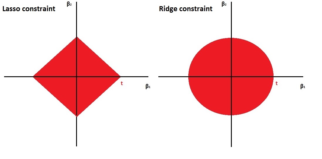
$Left: the constraint $|\beta_1| + |\beta_2| \leq t$, Right: the constraint $\beta_1^2 + \beta_2^2 \leq t$.$

Figure 4.3: Left: the constraint $|\beta_1| + |\beta_2| \leq t$, Right: the constraint $\beta_1^2 + \beta_2^2 \leq t$.

It is this difference between the smooth and edgy constraints that results in lasso having coefficient estimates that are exactly zero and ridge not. We illustrate this even further in Figure 4.4. The least squares solution is marked as $\hat{\beta}$, while the blue diamond and circle represent the lasso and ridge regression constraints (as in Figure 4.3). If $t$ is sufficiently large (making $t$ larger results in the diamond and circle respectively getting larger), then the constraint regions will contain $\hat{\beta}$, and so the ridge and lasso estimates will be the same as the least squares estimates.

The contours that are centered around $\hat{\beta}$ represent regions of constant RSS. As the ellipses expand away from the least squares coefficient estimates, the RSS increases. The lasso and ridge regression coefficient estimates are given by the first point at which an ellipse contacts the constraint region.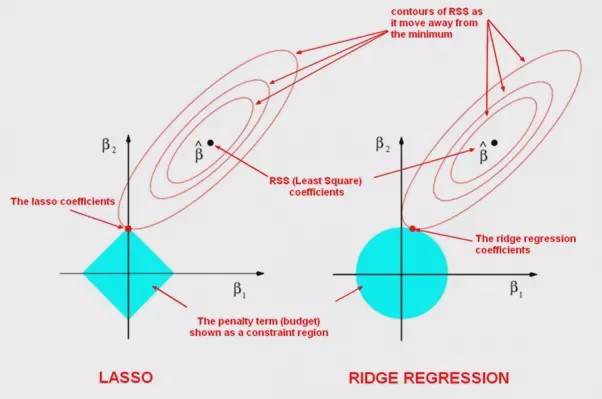

$Contours of the error and constraint functions for the lasso (left) and ridge regression (right). The solid blue areas are the constraint regions $|\beta_1| + |\beta_2| \leq t$ and $\beta_1^2 + \beta_2^2 \leq t$ respectively. The red ellipses are the contours of the Residual Sum of Squares, with the values along each contour being the same, and outer contours having a higher value (least squares $\hat{\beta}$ has minimal RSS).$

Figure 4.4: Contours of the error and constraint functions for the lasso (left) and ridge regression (right). The solid blue areas are the constraint regions $|\beta_1| + |\beta_2| \leq t$ and $\beta_1^2 + \beta_2^2 \leq t$ respectively. The red ellipses are the contours of the Residual Sum of Squares, with the values along each contour being the same, and outer contours having a higher value (least squares $\hat{\beta}$ has minimal RSS).

Since ridge regression has a circular constraint with no sharp points, this intersection will not generally occur on an axis, and so the ridge regression coefficient estimates will be exclusively non-zero. However, the lasso constraint has corners at each of the axes, and so the ellipse will often intersect the constraint region at an axis. When this occurs, one of the coefficient estimates will equal zero. In Figure 4.4, the intersection occurs at $\beta_1=0$, and so the resulting model will only include $\beta_2$.

4.3.3 Different $\lambda$’s

Both ridge and lasso are convex optimisation problems Boyd and Vandenberghe (2009).
In optimisation, convexity is a desired property.
In fact the ridge solution exists in closed form (meaning we have a formula for it, as we used in Section 3.3).
Lasso does not have a closed form solution, but nowadays there exist very efficient optimisation algorithms for the lasso solution.
Package glmnet in R implements coordinate descent (very fast) – same time to solve ridge and lasso.
Due to clever optimisation tricks, finding the solutions for multiple $\lambda$’s takes the same time as finding the solution for one single $\lambda$ value. This is very useful: it implies that we can obtain the solutions for a grid of values of $\lambda$ very fast and then pick a specific $\lambda$ that is optimal in regard to some objective function (see Chapter 5).

4.3.4 Predictive Performance

So, lasso has a clear advantage over ridge - it can set coefficients equal to zero!

This must mean that it is also better for prediction, right? Well, not necessarily. Things are a bit more complicated than that$...$it all comes down to the nature of the actual underlying mechanism. Lets explain this rather cryptic answer$...$

Generally…

When the actual data-generating mechanism is sparse lasso has the advantage.
When the actual data-generating mechanism is dense ridge has the advantage.

Sparse mechanisms: Few predictors are relevant to the response $\rightarrow$ good setting for lasso regression.

Dense mechanisms: A lot of predictors are relevant to the response $\rightarrow$ good setting for ridge regression.

Figure 4.5 roughly illustrates how prediction mean square error may depend on the density of the mechanism (number of predictors).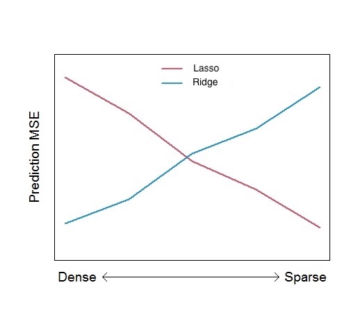

Figure 4.5: Rough illustration of the effect of mechanism density on prediction Mean Squared Error.

This figure really is a rough extreme illustration! The actual performance will also depend upon:

Signal strength (the magnitude of the effects of the relevant variables).
The correlation structure among predictors.
Sample size $n$ vs. number of predictors $p$.

4.3.5 So…which is better?

In general, none of the two shrinkage methods will dominate in terms of predictive performance under all settings.
Lasso performs better when few predictors have a substantial effect on the response variable.
Ridge performs better when a lot of predictors have a substantial effect on the response.
Keep in mind: a few and a lot are always relative to the total number of available predictors.
Overall: in most applications lasso is more robust.

Question: What should I do if I have to choose between ridge and lasso?

Answer: Keep a part of the data for testing purposes only and compare predictive performance of the two methods.

4.4 Practical Demonstration

We will continue analysing the Hitters dataset included in package ISLR, this time applying lasso regression.

4.4.1 Removing missing entries

We perform the usual steps of removing missing data as we have seen in previous practical demonstrations.

library(ISLR)
Hitters = na.omit(Hitters)
dim(Hitters)

## [1] 263  20

sum(is.na(Hitters))

## [1] 0

4.4.2 Lasso Regression

We will now use glmnet() to implement lasso regression.

library(glmnet)

Having learned how to implement ridge regression in Section 3.6 the analysis is very easy. To run lasso all we have to do is remove the option alpha = 0. We do not need to specify explicitly alpha = 1 because this is the default option in glmnet().

In this part again we call the response y and extract the matrix of predictors, which we call x using the command model.matrix().

y = Hitters$Salary
x = model.matrix(Salary~., Hitters)[,-1] # Here we exclude the first column 
                                         # because it corresponds to the 
                                         # intercept.
head(x)

##                   AtBat Hits HmRun Runs RBI Walks Years CAtBat CHits CHmRun CRuns CRBI
## -Alan Ashby         315   81     7   24  38    39    14   3449   835     69   321  414
## -Alvin Davis        479  130    18   66  72    76     3   1624   457     63   224  266
## -Andre Dawson       496  141    20   65  78    37    11   5628  1575    225   828  838
## -Andres Galarraga   321   87    10   39  42    30     2    396   101     12    48   46
## -Alfredo Griffin    594  169     4   74  51    35    11   4408  1133     19   501  336
## -Al Newman          185   37     1   23   8    21     2    214    42      1    30    9
##                   CWalks LeagueN DivisionW PutOuts Assists Errors NewLeagueN
## -Alan Ashby          375       1         1     632      43     10          1
## -Alvin Davis         263       0         1     880      82     14          0
## -Andre Dawson        354       1         0     200      11      3          1
## -Andres Galarraga     33       1         0     805      40      4          1
## -Alfredo Griffin     194       0         1     282     421     25          0
## -Al Newman            24       1         0      76     127      7          0

We then run lasso regression.

lasso = glmnet(x, y)

lambda and beta are still the most important components of the output.

names(lasso)

##  [1] "a0"        "beta"      "df"        "dim"       "lambda"    "dev.ratio" "nulldev"  
##  [8] "npasses"   "jerr"      "offset"    "call"      "nobs"

lasso$lambda

##  [1] 255.2820965 232.6035386 211.9396813 193.1115442 175.9560468 160.3245966 146.0818013
##  [8] 133.1042967 121.2796778 110.5055255 100.6885192  91.7436287  83.5933775  76.1671723
## [15]  69.4006906  63.2353245  57.6176726  52.4990774  47.8352040  43.5856563  39.7136268
## [22]  36.1855776  32.9709506  30.0419022  27.3730624  24.9413150  22.7255973  20.7067179
## [29]  18.8671902  17.1910810  15.6638727  14.2723374  13.0044223  11.8491453  10.7964999
## [36]   9.8373686   8.9634439   8.1671562   7.4416086   6.7805166   6.1781542   5.6293040
## [43]   5.1292121   4.6735471   4.2583620   3.8800609   3.5353670   3.2212947   2.9351238
## [50]   2.6743755   2.4367913   2.2203135   2.0230670   1.8433433   1.6795857   1.5303760
## [57]   1.3944216   1.2705450   1.1576733   1.0548288   0.9611207   0.8757374   0.7979393
## [64]   0.7270526   0.6624632   0.6036118   0.5499886   0.5011291   0.4566102   0.4160462
## [71]   0.3790858   0.3454089   0.3147237   0.2867645   0.2612891   0.2380769   0.2169268
## [78]   0.1976557   0.1800965   0.1640972

dim(lasso$beta)

## [1] 19 80

lasso$beta[,1:3]   # this returns only the predictor coefficients

## 19 x 3 sparse Matrix of class "dgCMatrix"
##            s0         s1         s2
## AtBat       . .          .         
## Hits        . .          .         
## HmRun       . .          .         
## Runs        . .          .         
## RBI         . .          .         
## Walks       . .          .         
## Years       . .          .         
## CAtBat      . .          .         
## CHits       . .          .         
## CHmRun      . .          .         
## CRuns       . .          0.01515244
## CRBI        . 0.07026614 0.11961370
## CWalks      . .          .         
## LeagueN     . .          .         
## DivisionW   . .          .         
## PutOuts     . .          .         
## Assists     . .          .         
## Errors      . .          .         
## NewLeagueN  . .          .

coef(lasso)[,1:3]  # this returns intercept + predictor coefficients

## 20 x 3 sparse Matrix of class "dgCMatrix"
##                   s0           s1           s2
## (Intercept) 535.9259 512.70866859 490.92996088
## AtBat         .        .            .         
## Hits          .        .            .         
## HmRun         .        .            .         
## Runs          .        .            .         
## RBI           .        .            .         
## Walks         .        .            .         
## Years         .        .            .         
## CAtBat        .        .            .         
## CHits         .        .            .         
## CHmRun        .        .            .         
## CRuns         .        .            0.01515244
## CRBI          .        0.07026614   0.11961370
## CWalks        .        .            .         
## LeagueN       .        .            .         
## DivisionW     .        .            .         
## PutOuts       .        .            .         
## Assists       .        .            .         
## Errors        .        .            .         
## NewLeagueN    .        .            .

We see that as expected lasso$beta has 19 rows (number of predictors) and 80 columns (length of the grid). Using coef instead includes the intercept term. The key difference this time (in comparison to the application to ridge regression in Section 3.6) is that some of the elements of the output are replaced with a “.”, indicating that the corresponding predictor is not included in the lasso regression model with that value of $\lambda$.

We now produce a 1 by 2 plot displaying on the left regularisation paths based on $\log\lambda$ and on the right the paths based on the $\ell_1$-norm. The numbers along the top now correspond to the number of predictors in the model for the corresponding (log) $\lambda$ and $\ell_1$-norm values respectively. Recall the row of 19’s across the top of the corresponding plot for ridge regression - this is because for ridge we always include all predictors.

par(mfrow=c(1, 2))
plot(lasso, xvar = 'lambda')
plot(lasso, xvar = 'norm')  # or simply plot(lasso) because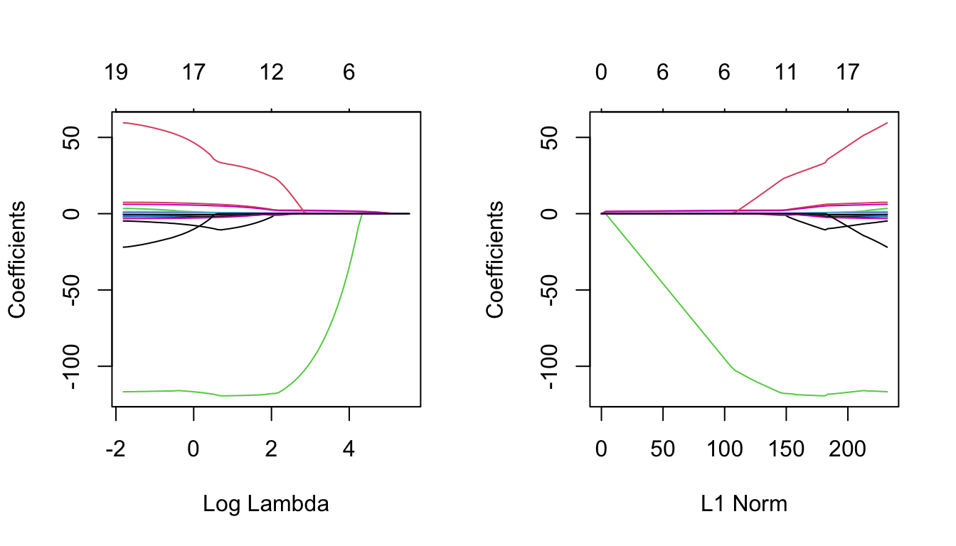

                            # xvar = 'norm' is the default.

References

Boyd, S., and L. Vandenberghe. 2009. Convex Optimization. 7th ed. Cambridge: Cambridge University Press.

James, G., D. Witten, T. Hastie, and R. Tibshirani. 2013. An Introduction to Statistical Learning. Edited by G. Casella, Fienberg S, and I. Olkin. New York: Springer.

Note: Some of the figures in these notes are taken from James et al. (2013) with permission from the authors: G. James, D. Witten, T. Hastie and R. Tibshirani.↩︎

Machine Learning