Practical 3 Solutions
Make sure to at least finish Practical 1 before continuing with this practical! It might be tempting to skip some stuff if you’re behind, but you may end up more lost\(...\)we will happily answer questions from any previous practical each session.
We continue analysing the fat data in package faraway in this practical. Run the following commands to load the package and obtain our reduced dataset fat1 of interest. We also load the glmnet package for performing ridge regression.
library(faraway)
fat1 <- fat[,-c(2, 3, 8)]
library(glmnet)
Q1 Ridge Regression
- Define a vector
ycontaining all the values of the response variablebrozek.
y = fat1$brozek- Stack the predictors column-wise into a matrix, and define this matrix as
x.
x = model.matrix(brozek~., fat1)[,-1]- Fit a model of the predictors for the response using ridge regression over a grid of 200 \(\lambda\) values. Hint: type
?glmnetand look at argumentnlambda.
ridge = glmnet(x, y, alpha = 0, nlambda = 200)- Plot the regularisation paths of the ridge regresssion coefficients as a function of log \(\lambda\).
plot(ridge, xvar = 'lambda')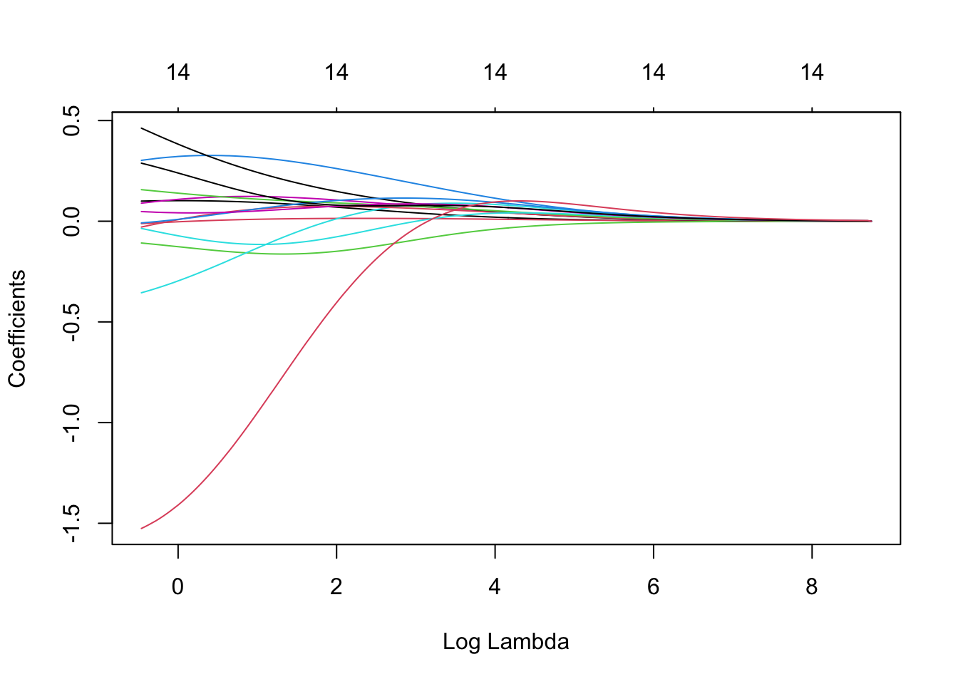
Q2 Cross-Validation
- Using
cv.glmnetwith 5-fold CV and random seed equal to 2, find the values of min-CV \(\lambda\) and 1-se \(\lambda\).
set.seed(2)
ridge.cv = cv.glmnet(x, y, alpha=0, nfolds = 5)
ridge.cv$lambda.min
## [1] 0.6294393ridge.cv$lambda.1se## [1] 1.454086- Plot the CV \(\lambda\) graph next to the regularisation-path plot indicating with vertical lines the two \(\lambda\) values.
par(mfrow=c(1,2))
plot(ridge.cv)
plot(ridge, xvar = 'lambda')
abline(v = log(ridge.cv$lambda.min), lty = 3)
abline(v = log(ridge.cv$lambda.1se), lty = 3)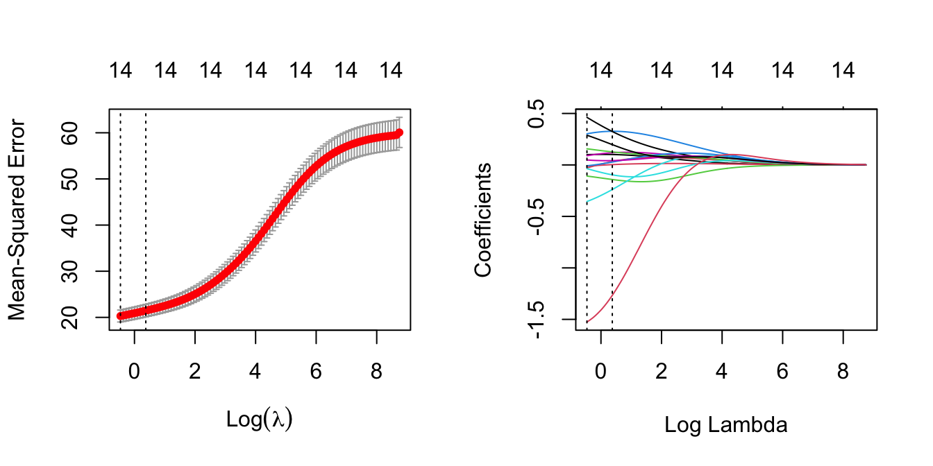
- Which predictor has the highest absolute coefficient?
abs(coef(ridge.cv))## 15 x 1 sparse Matrix of class "dgCMatrix"
## s1
## (Intercept) 11.084963486
## age 0.101081788
## weight 0.002854877
## height 0.141616551
## adipos 0.325547676
## neck 0.239066118
## chest 0.118435588
## abdom 0.324829169
## hip 0.033194250
## thigh 0.127019937
## knee 0.028284305
## ankle 0.095625648
## biceps 0.042553472
## forearm 0.197620295
## wrist 1.265884058# it is wrist for 1-se lambda
abs(coef(ridge.cv, s ='lambda.min'))## 15 x 1 sparse Matrix of class "dgCMatrix"
## s1
## (Intercept) 9.174745514
## age 0.099911854
## weight 0.012172773
## height 0.108068586
## adipos 0.301584522
## neck 0.354687819
## chest 0.089843263
## abdom 0.462355382
## hip 0.028571052
## thigh 0.156802210
## knee 0.007910553
## ankle 0.035339905
## biceps 0.048198960
## forearm 0.288207387
## wrist 1.525865471# it is also wrist for min-CV lambda- Type
plot(ridge.cv)into the R console. What is plotted?
plot(ridge.cv)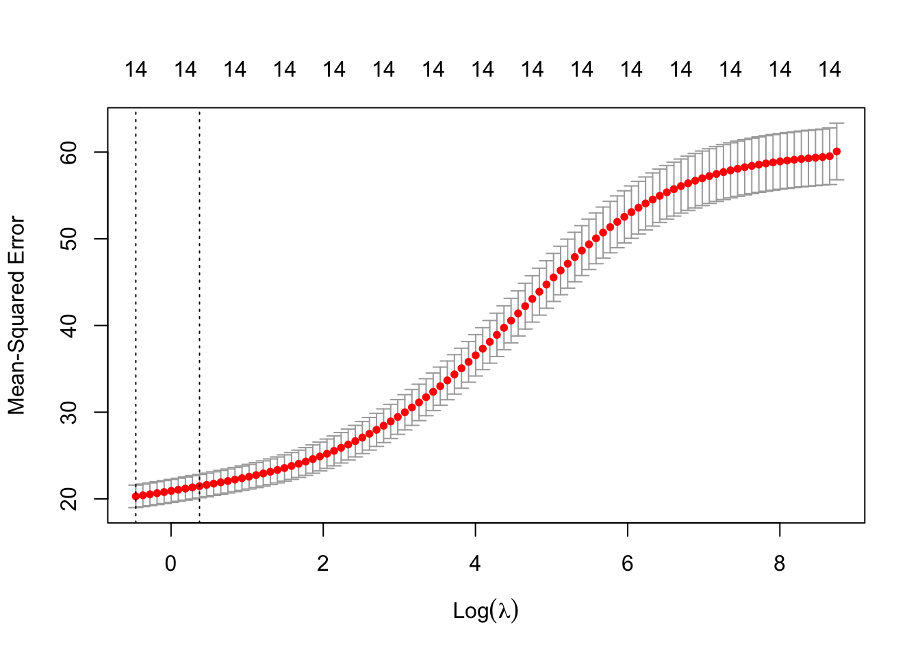
# We see the estimated CV MSE for each value of log lambda, along with
# the 1 standard error interval bars of those estimates.
# The vertical lines show the min-CV lambda and 1-se lambda values.
Q3 Comparison of Predictive Performance
Using 50 repetitions with random seed set to 2, compare whether the model with min-CV \(\lambda\) or 1-se \(\lambda\) may be preferable in terms of predictive performance. In this case use 5-fold CV within cv.glmnet() and also a 50% splitting for training and testing. Produce boxplots of the correlation values obtained from each cycle of your for loop. Finally, calculate the mean correlations from the two models. Under which approach does ridge seem to perform better?
repetitions = 50
cor.1 = c()
cor.2 = c()

set.seed(2)
for(i in 1:repetitions){
  # Step (i) data splitting
  training.obs = sample(1:252,  126)
  y.train = fat1$brozek[training.obs]
  x.train = model.matrix(brozek~., fat1[training.obs, ])[,-1]
  y.test = fat1$brozek[-training.obs]
  x.test = model.matrix(brozek~., fat1[-training.obs, ])[,-1]

  # Step (ii) training phase
  ridge.train = cv.glmnet(x.train, y.train, alpha = 0, nfolds = 5)

  # Step (iii) generating predictions
  predict.1 = predict(ridge.train, x.test, s = 'lambda.min')
  predict.2 = predict(ridge.train, x.test, s = 'lambda.1se')

  # Step (iv) evaluating predictive performance
  cor.1[i] = cor(y.test, predict.1)
  cor.2[i] = cor(y.test, predict.2)
}

boxplot(cor.1, cor.2, names = c('Ridge min-CV lambda','Ridge 1-se lambda'),
        ylab = 'Test correlation', col = 3)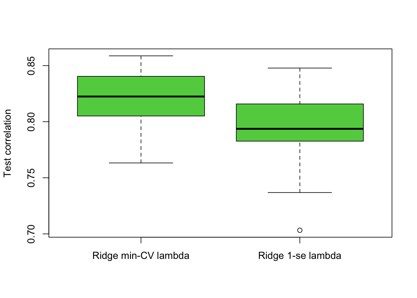
mean(cor.1)## [1] 0.8204005mean(cor.2)## [1] 0.796162# Ridge regression based on min-CV lambda seems to be better.