Practical 2 Solutions
Make sure to finish Practical 1 before continuing with this practical! It might be tempting to skip some stuff if you’re behind, but you may end up more lost\(...\)we will happily answer questions from any previous practical each session.
In this practical, we continue our analysis of the fat data in library faraway introduced in Practical 1. Before starting, run the following commands to obtain our reduced dataset of interest, fat1, as you should have defined in Question 1(d) of Practical 1. We also load library leaps for function regsubsets later.
library("leaps")
library("faraway")
fat1 <- fat[,-c(2, 3, 8)]
Q1 Predictive Performance
- Based on forward selection, evaluate the predictive accuracy (using validation mean squared errors) of models with numbers of predictors ranging from 1 to 14 based on a training and test sample. Use approximately 75% of the samples for training. You can use the
predict.regsubsetsfunction defined in practical demonstration Section 2.4.4. To make the results of your answer to this part reproducible (and in line with the published solutions), include the lineset.seed(1)at the top of your code to set the random seed number equal to 1.
# Set the seed so that the results are reproducible.
set.seed(1)

# We use this function for prediction.
predict.regsubsets = function(object, newdata, id, ...){
  form = as.formula(object$call[[2]])
  mat = model.matrix(form, newdata)
  coefi = coef(object, id = id)
  xvars = names(coefi)
  mat[, xvars]%*%coefi
}nrow(fat) # Number of rows (samples) in the dataset.## [1] 252# 252
# Use 3/4 of the samples for training.
training.obs <- sample( 1:252, 189 )
fat.train <- fat1[training.obs,]
fat.test = fat1[-training.obs, ]
# Apply regsubsets() to the training set,
fwd = regsubsets(brozek~., method = "forward", data = fat.train, nvmax = 14)
# Use a for loop to store the validation mean squared errors of each model
# in a vector.
val.error <- c()
for( i in 1:14 ){
pred = predict.regsubsets( fwd, fat.test, i )
val.error[i] = mean( ( fat.test$brozek - pred )^2 )
}
# Let's have a look at the validation error results.
val.error## [1] 23.63794 17.96604 18.54564 19.61482 19.48348 19.02309 18.38694 18.81967 19.60463
## [10] 19.62195 19.49129 19.74260 19.64187 19.63980- How many predictors are included in the model which is optimal based on the validation mean squared errors obtained for the particular splitting of training and test data used in part (a)? Which predictors are they?
# Find how many predictors the model with minimum mean squared validation
# error has.
which.min( val.error )
## [1] 2# The optimal model based on minimum mean squared validation error under
# this splitting of the data has only two predictors.
coef( fwd, 2 )## (Intercept) weight abdom
## -40.2273453 -0.1283838 0.8862161# They are weight and abdom.Whilst we set the seed number equal to 1 in part (a), you should also play around with changing the seed number and investigating whether the sampling randomness of training and test data affects your results. This is the focus of parts (c) and (d).
- Change the seed number in part (a) to 67 and repeat the analysis. Does this affect the results?
# Set the seed so that the results are reproducible.
set.seed(67)

# Use 3/4 of the samples for training.
training.obs <- sample( 1:252, 189 )
fat.train <- fat1[training.obs,]
fat.test = fat1[-training.obs, ]

# Apply regsubsets() to the training set,
fwd = regsubsets(brozek~., method = "forward", data = fat.train, nvmax = 14)

# Use a for loop to store the validation mean squared errors of
# each model in a vector.
val.error <- c()
for( i in 1:14 ){
  pred = predict.regsubsets( fwd, fat.test, i )
  val.error[i] = mean( ( fat.test$brozek - pred )^2 )
}

# Let's have a look at the validation error results.
val.error
## [1] 22.93834 20.54789 19.85644 19.41615 20.02322 22.85582 22.30972 22.45490 20.61842
## [10] 19.65655 19.79789 19.89627 19.86825 19.89914# Find how many predictors the model with
# minimum mean squared validation error has.
which.min( val.error )## [1] 4# The optimal model based on minimum mean squared validation error
# under this splitting of the data has four predictors.
coef( fwd, 4 )## (Intercept) age height abdom wrist
## -2.36221453 0.07096607 -0.13766321 0.69246862 -1.98491762# They are age, height, abdom and wrist.
# We can therefore see that using a different training and test data split
# has resulted in more predictors, and different predictors.
# Only abdom is similar across both optimal models.- Finally, we investigate the spread in the number of predictors chosen for many different splits of training and test data, such as was carried out for the
Hittersdata in Section 2.4.6. Loop over the forward stepwise selection analysis of part (a) for seed numbers 1 to 100, storing the number of predictors that are chosen in each case in a vector. Display the results in a histogram.
min.valid = c()

for(n in 1:100){
  set.seed(n)
  training.obs = sample(1:252, 189)
  fat.train = fat1[training.obs,  ]
  fat.test = fat1[-training.obs,  ]

  fwd = regsubsets(brozek~., method="forward", data = fat.train, nvmax = 14)

  val.error<-c()
  for(i in 1:14){
    pred = predict.regsubsets(fwd, fat.test, i)
    val.error[i] = mean((fat.test$brozek - pred)^2)
  }
  val.error
  min.valid[n] = which.min(val.error)
}

hist(min.valid, col = 3, breaks = seq( from = 0.5, to = 14.5, length = 15 ),
     xlab = 'Number of Predictors', main = 'BSS with validation')
abline(v = mean(min.valid), col = 2, lwd = 4)
legend('topright', legend=c('Average selection'),bty = 'n', lty = 1,
       lwd = 4, col = 2)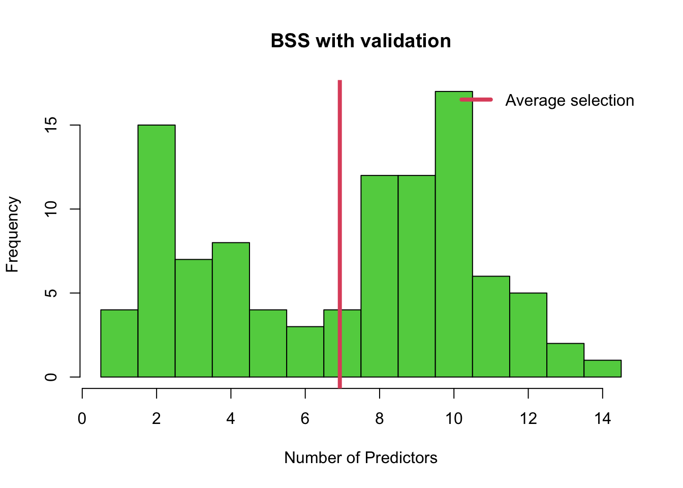
# We can also use tabulate to see these values numerically.
tabulate( min.valid )
## [1] 4 15 7 8 4 3 4 12 12 17 6 5 2 1Q2 Cross-Validation
Using a similar approach to that discussed in Section 2.4.7, compare the 5-fold cross-validated predictive accuracy of the two models with i) minimum \(C_p\), ii) minimum BIC, using the whole dataset under forwards stepwise selection (in other words, those found in Practical 1, Q3c). Which model does this analysis suggest that you use? For reproducibility purposes, and to make your answer in line with the published solutions, it is recommended to include the line set.seed(1) before generating the random folds.
# Perform forwards stepwise selection using the entire dataset.
fwd = regsubsets(brozek~., data = fat1, method = 'forward', nvmax = 14)

# Summary of the relevant commands and results of Practical 1, Q3c.
results = summary(fwd)
Cp = results$cp
BIC = results$bic
which.min(Cp)
## [1] 8which.min(BIC) ## [1] 4# The optimal models had 4 (min BIC) and 8 (min Cp) predictors.
coef(fwd, 4) # weight, abdom, forearm and wrist.## (Intercept) weight abdom forearm wrist
## -31.2967858 -0.1255654 0.9213725 0.4463824 -1.3917662coef(fwd, 8) # in addition age, neck, hip and thigh.## (Intercept) age weight neck abdom hip
## -20.06213373 0.05921577 -0.08413521 -0.43189267 0.87720667 -0.18641032
## thigh forearm wrist
## 0.28644340 0.48254563 -1.40486912# Create 5 folds.
k = 5
folds = cut(seq(1, 252), breaks=k, labels=FALSE)
# Set the random seed number before random splitting of data for
# reproducibility purposes.
set.seed(1)
folds <- sample(folds) # random reshuffle of data.
# Create a matrix with 5 rows and 2 columns to store the results
# of cross-validation.
cv.errors = matrix(NA, nrow = k, ncol = 2,
dimnames = list(NULL, c("ls4", "ls8")))
# Loop over the folds - each time fitting a linear model with all data
# except fold i using lm, and predicting model output for the data in
# fold i.
for(i in 1:k){
ls4 = lm(brozek ~ weight + abdom + forearm + wrist, data = fat[folds!=i,] )
ls8 = lm(brozek ~ weight + abdom + forearm + wrist
+ age + neck + hip + thigh, data = fat[folds!=i,] )
pred4 <- predict( ls4, newdata = fat[folds==i, ] )
pred8 <- predict( ls8, newdata = fat[folds==i, ] )
cv.errors[i,] = c( mean( (fat$brozek[folds==i]-pred4)^2),
mean( (fat$brozek[folds==i]-pred8)^2) )
}
# Print the result.
cv.errors## ls4 ls8
## [1,] 18.86796 18.32572
## [2,] 17.82873 18.16430
## [3,] 17.88805 18.07617
## [4,] 13.59515 12.07325
## [5,] 16.54698 17.01779# Take the average of the MSEs in each column of the matrix.
cv.mean.errors <- colMeans(cv.errors)
cv.mean.errors## ls4 ls8
## 16.94537 16.73145# We may select model ls8, corresponding to the model with 8 predictors and
# that with minimum Cp, as it has a slightly lower average cross-validation
# error. On the other hand, since the difference is only small, we could
# pick ls4 as it has fewer predictors and thus is likely to be more
# interpretable.