Practical 5 Solutions
In this practical we consider two datasets for analysis by polynomial and step-wise function regression. Firstly the seatpos dataset analysed in Practical 4, followed by the Boston data analysed in practical demonstration Section 7.4.
Q1 seatpos Data
- Load libraries
MASSandfaraway.
library("MASS")
library("faraway")- We will analyse the effects of predictor variable
Hton the response variablehipcenter. Assign thehipcentervalues to a vectory, and theHtvariable values to a vectorx.
y = seatpos$hipcenter
x = seatpos$Ht- Plot variable
Htandhipcenteragainst each other. Remember to include suitable axis labels. From visual inspection of this plot, what sort of polynomial might be appropriate for this data?
y.lab = 'hip center (mm)'
x.lab = 'Height (bare foot) in cm'
plot( x, y, cex.lab = 1.1, col="darkgrey", xlab = x.lab, ylab = y.lab,
      main = "", bty = 'l', pch = 16 )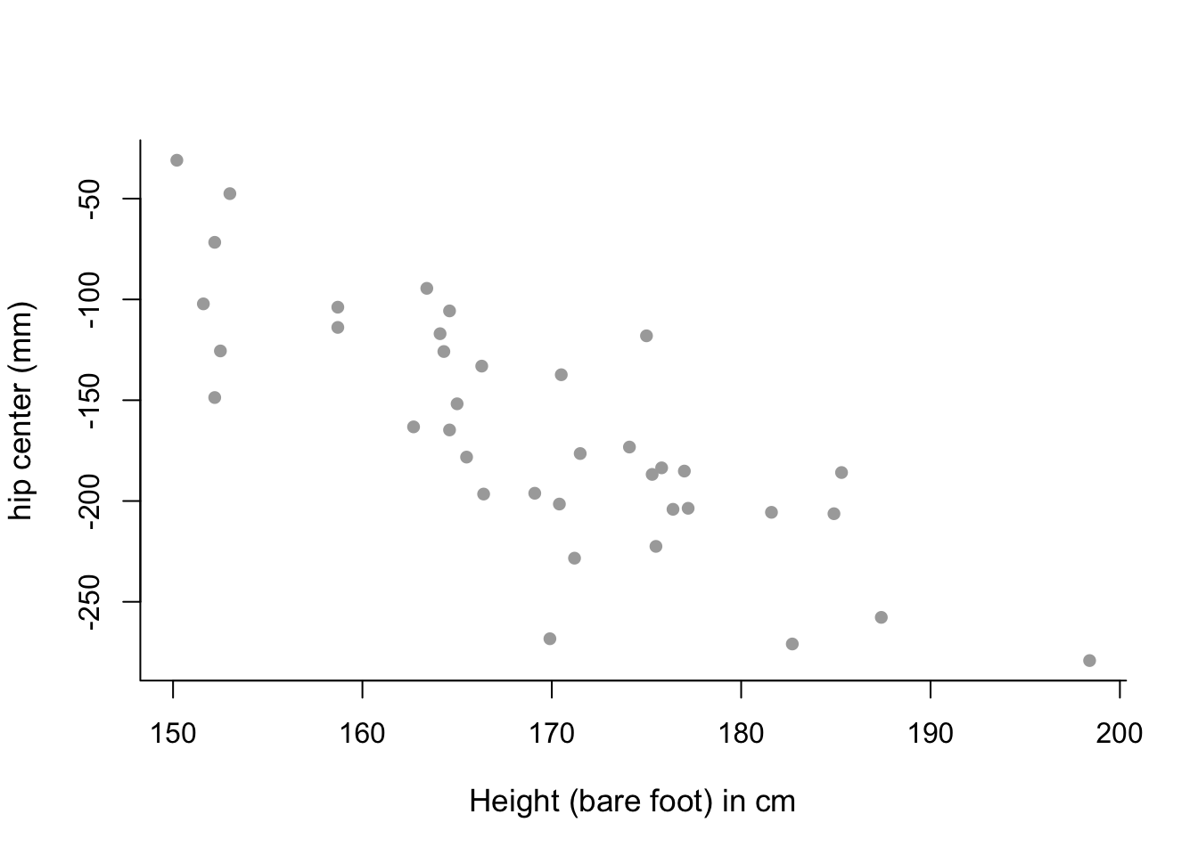
# mean trend in the data looks almost linear - perhaps only a
# first-order polynomial model is needed.- Fit a first and second order polynomial to the data using the commands
lmandpoly. Look at the corresponding summary objects. Do these back up your answer to part (c)?
poly1 = lm(y ~ poly(x,  1))
summary(poly1)
##
## Call:
## lm(formula = y ~ poly(x, 1))
##
## Residuals:
## Min 1Q Median 3Q Max
## -99.956 -27.850 5.656 20.883 72.066
##
## Coefficients:
## Estimate Std. Error t value Pr(>|t|)
## (Intercept) -164.88 5.90 -27.95 < 2e-16 ***
## poly(x, 1) -289.87 36.37 -7.97 1.83e-09 ***
## ---
## Signif. codes: 0 '***' 0.001 '**' 0.01 '*' 0.05 '.' 0.1 ' ' 1
##
## Residual standard error: 36.37 on 36 degrees of freedom
## Multiple R-squared: 0.6383, Adjusted R-squared: 0.6282
## F-statistic: 63.53 on 1 and 36 DF, p-value: 1.831e-09poly2 = lm(y ~ poly(x, 2))
summary(poly2)##
## Call:
## lm(formula = y ~ poly(x, 2))
##
## Residuals:
## Min 1Q Median 3Q Max
## -96.068 -25.018 4.418 22.790 75.322
##
## Coefficients:
## Estimate Std. Error t value Pr(>|t|)
## (Intercept) -164.885 5.919 -27.855 < 2e-16 ***
## poly(x, 2)1 -289.868 36.490 -7.944 2.42e-09 ***
## poly(x, 2)2 31.822 36.490 0.872 0.389
## ---
## Signif. codes: 0 '***' 0.001 '**' 0.01 '*' 0.05 '.' 0.1 ' ' 1
##
## Residual standard error: 36.49 on 35 degrees of freedom
## Multiple R-squared: 0.646, Adjusted R-squared: 0.6257
## F-statistic: 31.93 on 2 and 35 DF, p-value: 1.282e-08# p-value for second order term is high, suggesting that it is not
# necessary in the model. This backs up our conclusion to part (c).- Plot the first and second polynomial fits to the data, along with \(\pm2\) standard deviation confidence intervals, similar to those generated in practical demonstration Section 7.4. What do you notice about the degree-2 polynomial plot?
sort.x = sort(x) # sorted values of x.

# Predicted values.
pred1 = predict(poly1, newdata = list(x = sort.x), se = TRUE)
pred2 = predict(poly2, newdata = list(x = sort.x), se = TRUE)

# Confidence interval bands.
se.bands1 = cbind( pred1$fit - 2*pred1$se.fit, pred1$fit + 2*pred1$se.fit )
se.bands2 = cbind( pred2$fit - 2*pred2$se.fit, pred2$fit + 2*pred2$se.fit )

# Plot both plots on a single graphics device.
par(mfrow = c(1,2))

# Degree-1 polynomial plot.
plot(x, y, cex.lab = 1.1, col="darkgrey", xlab = x.lab, ylab = y.lab,
     main = "Degree-1 polynomial", bty = 'l')
lines(sort.x, pred1$fit, lwd = 2, col = "red")
matlines(sort.x, se.bands1, lwd = 2, col = "red", lty = 3)

# Degree-2 polynomial plot.
plot(x, y, cex.lab = 1.1, col="darkgrey", xlab = x.lab, ylab = y.lab,
     main = "Degree-2 polynomial", bty = 'l')
lines(sort.x, pred2$fit, lwd = 2, col = "red")
matlines(sort.x, se.bands2, lwd = 2, col = "red", lty = 3)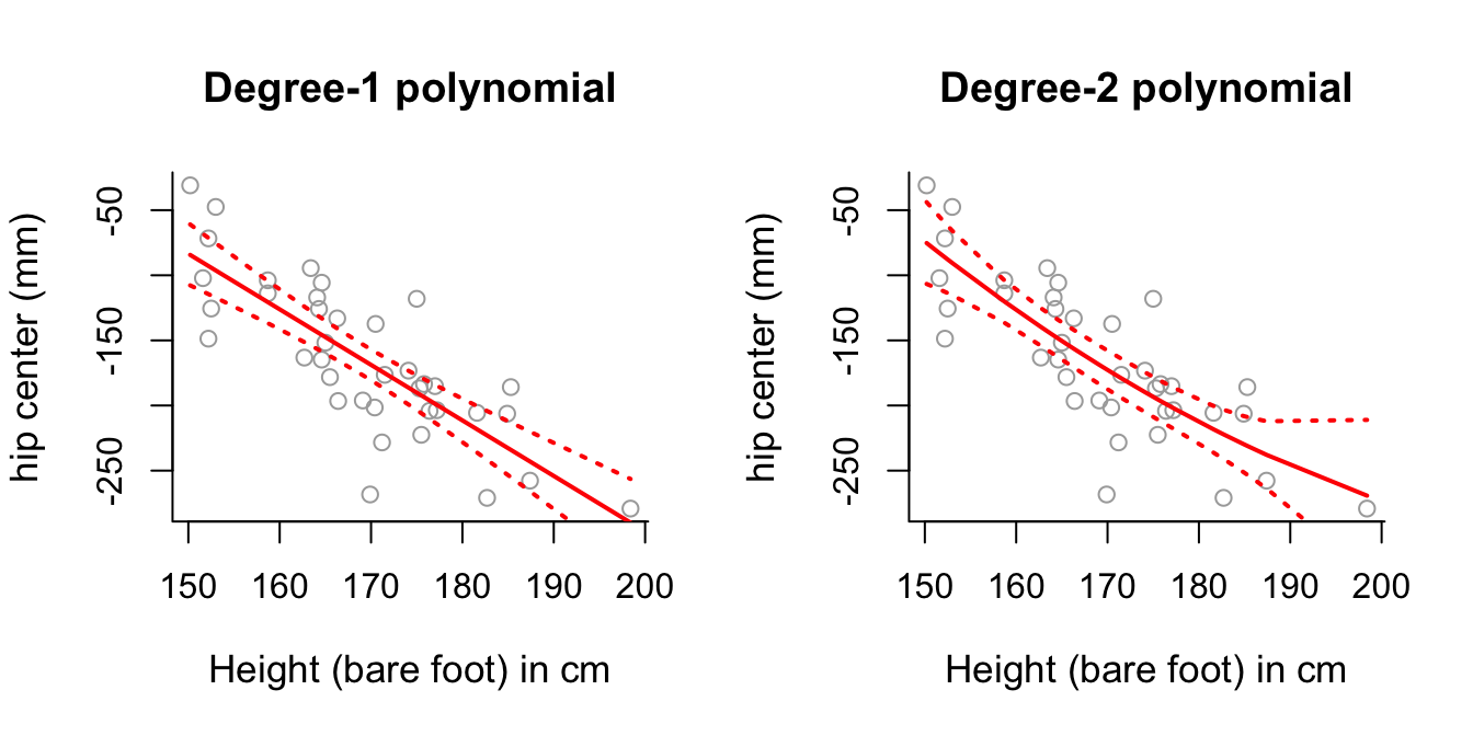
# Degree-2 polynomial plot looks relatively close to a straight line as
# well - perhaps this suggests the second order component isn't necessary?- Perform an analysis of variance to confirm whether higher order degrees of polynomial are useful for modelling
hipcenterbased onHt.
# Degree-3 and 4 polynomials.
poly3 = lm(y ~ poly(x,  3))
poly4 = lm(y ~ poly(x,  4))
anova(poly1, poly2, poly3, poly4)
## Analysis of Variance Table
##
## Model 1: y ~ poly(x, 1)
## Model 2: y ~ poly(x, 2)
## Model 3: y ~ poly(x, 3)
## Model 4: y ~ poly(x, 4)
## Res.Df RSS Df Sum of Sq F Pr(>F)
## 1 36 47616
## 2 35 46603 1 1012.64 0.7250 0.4006
## 3 34 46445 1 157.91 0.1131 0.7388
## 4 33 46093 1 352.27 0.2522 0.6189# Results suggest that use of the first-order polynomial is sufficient,
# which confirms the results of the previous parts of this question.- Use step function regression with 5 cut-points to model
hipcenterbased onHt. Plot the results.
# Remember to define the number of intervals (one more than the number of
# cut-points).
step6 = lm(y ~ cut(x, 6))
pred6 = predict(step6, newdata = list(x = sort(x)), se = TRUE)
se.bands6 = cbind(pred6$fit + 2*pred6$se.fit, pred6$fit-2*pred6$se.fit)

# Plot the results.
plot(x, y, cex.lab = 1.1, col="darkgrey", xlab = x.lab, ylab = y.lab,
     main = "5 cutpoints", bty = 'l')
lines(sort(x), pred6$fit, lwd = 2, col = "red")
matlines(sort(x), se.bands6, lwd = 1.4, col = "red", lty = 3)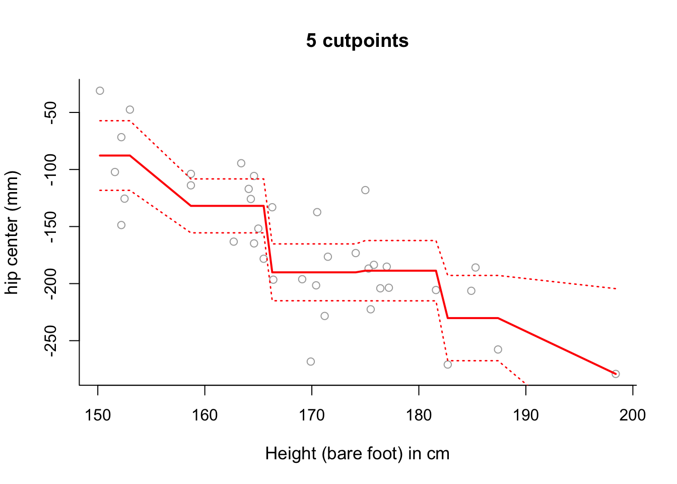
# Note that the slopes in this plot are an artifact of the way in which we
# have plotted the results.
# Use summary to see where the different intervals start and finish.
summary(step6)
##
## Call:
## lm(formula = y ~ cut(x, 6))
##
## Residuals:
## Min 1Q Median 3Q Max
## -78.209 -25.615 0.936 22.425 70.623
##
## Coefficients:
## Estimate Std. Error t value Pr(>|t|)
## (Intercept) -87.76 15.25 -5.753 2.22e-06 ***
## cut(x, 6)(158,166] -44.11 19.29 -2.286 0.029 *
## cut(x, 6)(166,174] -102.35 19.69 -5.197 1.12e-05 ***
## cut(x, 6)(174,182] -100.91 20.18 -5.001 1.98e-05 ***
## cut(x, 6)(182,190] -142.44 24.12 -5.906 1.43e-06 ***
## cut(x, 6)(190,198] -191.39 40.36 -4.742 4.20e-05 ***
## ---
## Signif. codes: 0 '***' 0.001 '**' 0.01 '*' 0.05 '.' 0.1 ' ' 1
##
## Residual standard error: 37.36 on 32 degrees of freedom
## Multiple R-squared: 0.6606, Adjusted R-squared: 0.6076
## F-statistic: 12.46 on 5 and 32 DF, p-value: 9.372e-07# The fitted model can be more accurately fitted over the data as follows:
newx <- seq(from = min(x), to = max(x), length = 100)
pred6 = predict(step6, newdata = list(x = newx), se = TRUE)
se.bands6 = cbind(pred6$fit + 2*pred6$se.fit, pred6$fit-2*pred6$se.fit)
plot(x, y, cex.lab = 1.1, col="darkgrey", xlab = x.lab, ylab = y.lab,
main = "5 cutpoints", bty = 'l')
lines(newx, pred6$fit, lwd = 2, col = "red")
matlines(newx, se.bands6, lwd = 1.4, col = "red", lty = 3)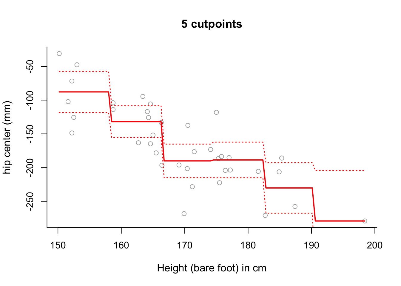
# Whilst there is still some sloping artifact to the plot, it is more
# negligible now - that is, the plot of the fitted values more accurately
# represents the step-wise nature of the model.
# Note that this was also present in the examples in
# Section 8.1 and 8.2 - but less noticable due to the amount of data.
# Change length = 1000 in the command seq for newx and you will see the
# steps become more step-like still!
Q2 Boston Data
The relationship between predictor indus and response medv of the Boston data also looks interesting. Predictor indus is the proportion of non-retail business acres per town. First plot the variables to see how the relationship between indus and medv looks like. Then analyse the data. Feel free to select between polynomials and step functions (of course you can experiment with both if you have time). If you use step functions you can also choose to define the intervals manually if you so wish. Use ANOVA to decide which model fits the data best.
library(MASS)
?Boston
sum(is.na(Boston))
## [1] 0names(Boston)## [1] "crim" "zn" "indus" "chas" "nox" "rm" "age" "dis"
## [9] "rad" "tax" "ptratio" "black" "lstat" "medv"head(Boston)## crim zn indus chas nox rm age dis rad tax ptratio black lstat medv
## 1 0.00632 18 2.31 0 0.538 6.575 65.2 4.0900 1 296 15.3 396.90 4.98 24.0
## 2 0.02731 0 7.07 0 0.469 6.421 78.9 4.9671 2 242 17.8 396.90 9.14 21.6
## 3 0.02729 0 7.07 0 0.469 7.185 61.1 4.9671 2 242 17.8 392.83 4.03 34.7
## 4 0.03237 0 2.18 0 0.458 6.998 45.8 6.0622 3 222 18.7 394.63 2.94 33.4
## 5 0.06905 0 2.18 0 0.458 7.147 54.2 6.0622 3 222 18.7 396.90 5.33 36.2
## 6 0.02985 0 2.18 0 0.458 6.430 58.7 6.0622 3 222 18.7 394.12 5.21 28.7y = Boston$medv
x = Boston$indus
y.lab = 'Median Property Value'
x.lab = 'Non-retail business acres per town'
# Plot the data for initial visual analysis.
plot(x, y, cex.lab = 1.1, col="darkgrey", xlab = x.lab, ylab = y.lab,
main = "", bty = 'l')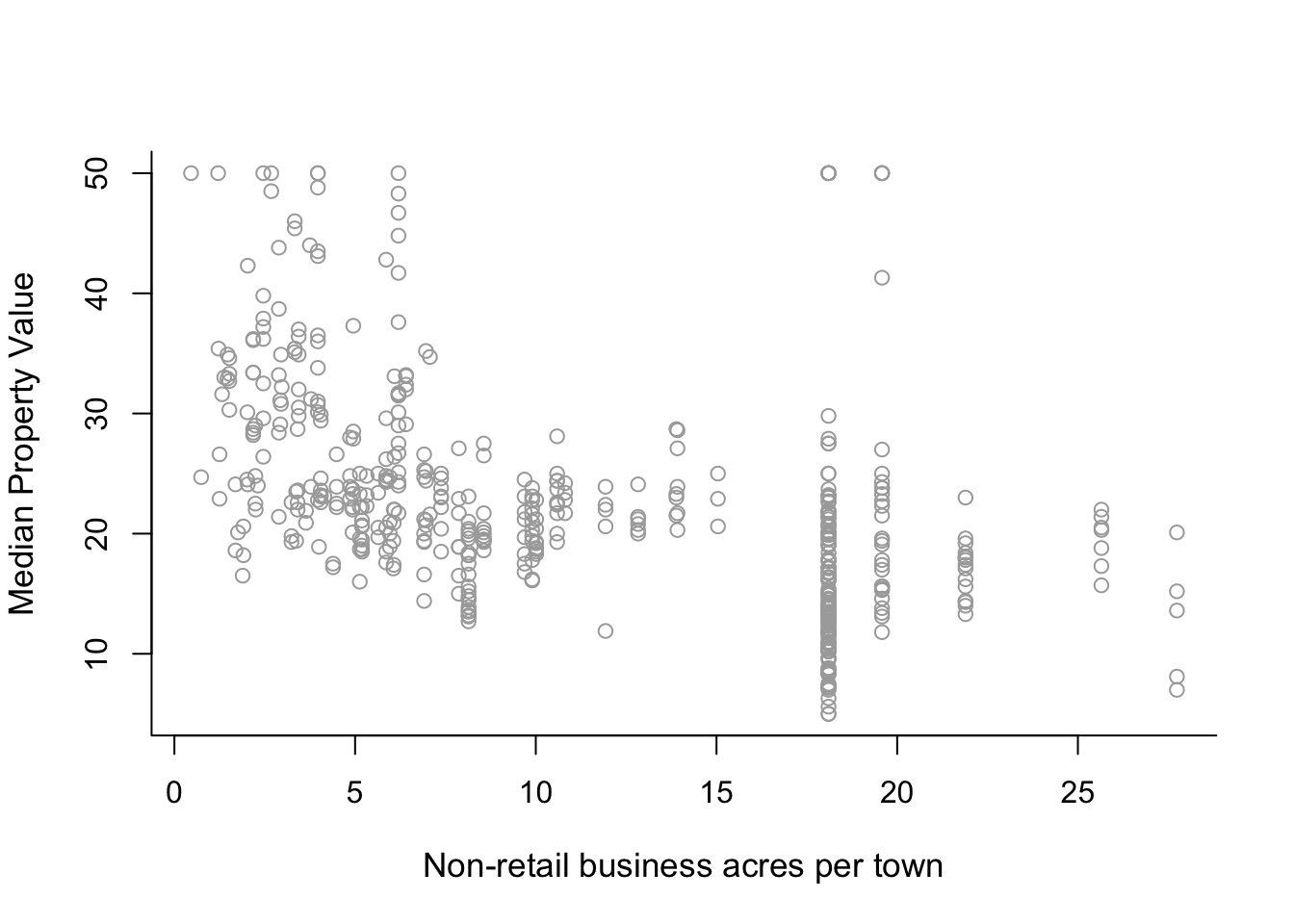
# Fit a second-order polynomial model.
poly2 = lm(y ~ poly(x,  2))

sort.x = sort(x)
sort.x[1:10]     # the first 10 sorted values of x
## [1] 0.46 0.74 1.21 1.22 1.25 1.25 1.32 1.38 1.47 1.47pred2 = predict(poly2, newdata = list(x = sort.x), se = TRUE)
names(pred2)## [1] "fit" "se.fit" "df" "residual.scale"# plus/minus 2 standard deviation confidence intervals.
se.bands2 = cbind(pred2$fit + 2 * pred2$se.fit, pred2$fit - 2 * pred2$se.fit)
pred2$fit[1:10] # the first 10 fitted values of the curve## 1 2 3 4 5 6 7 8 9
## 33.37033 32.90299 32.13412 32.11798 32.06959 32.06959 31.95699 31.86083 31.71718
## 10
## 31.71718se.bands2[1:10,] # the first 10 confidence intervals of the curve## [,1] [,2]
## 1 35.43113 31.30952
## 2 34.85860 30.94738
## 3 33.92209 30.34615
## 4 33.90251 30.33345
## 5 33.84383 30.29535
## 6 33.84383 30.29535
## 7 33.70740 30.20658
## 8 33.59102 30.13063
## 9 33.41742 30.01694
## 10 33.41742 30.01694# Plot the fitted degree-2 polynomial along with 2 standard deviation
# confidence interval errors.
plot(x, y, cex.lab = 1.1, col="darkgrey", xlab = x.lab, ylab = y.lab,
main = "Degree-2 polynomial", bty = 'l')
lines(sort.x, pred2$fit, lwd = 2, col = "red")
matlines(sort.x, se.bands2, lwd = 1.4, col = "red", lty = 3)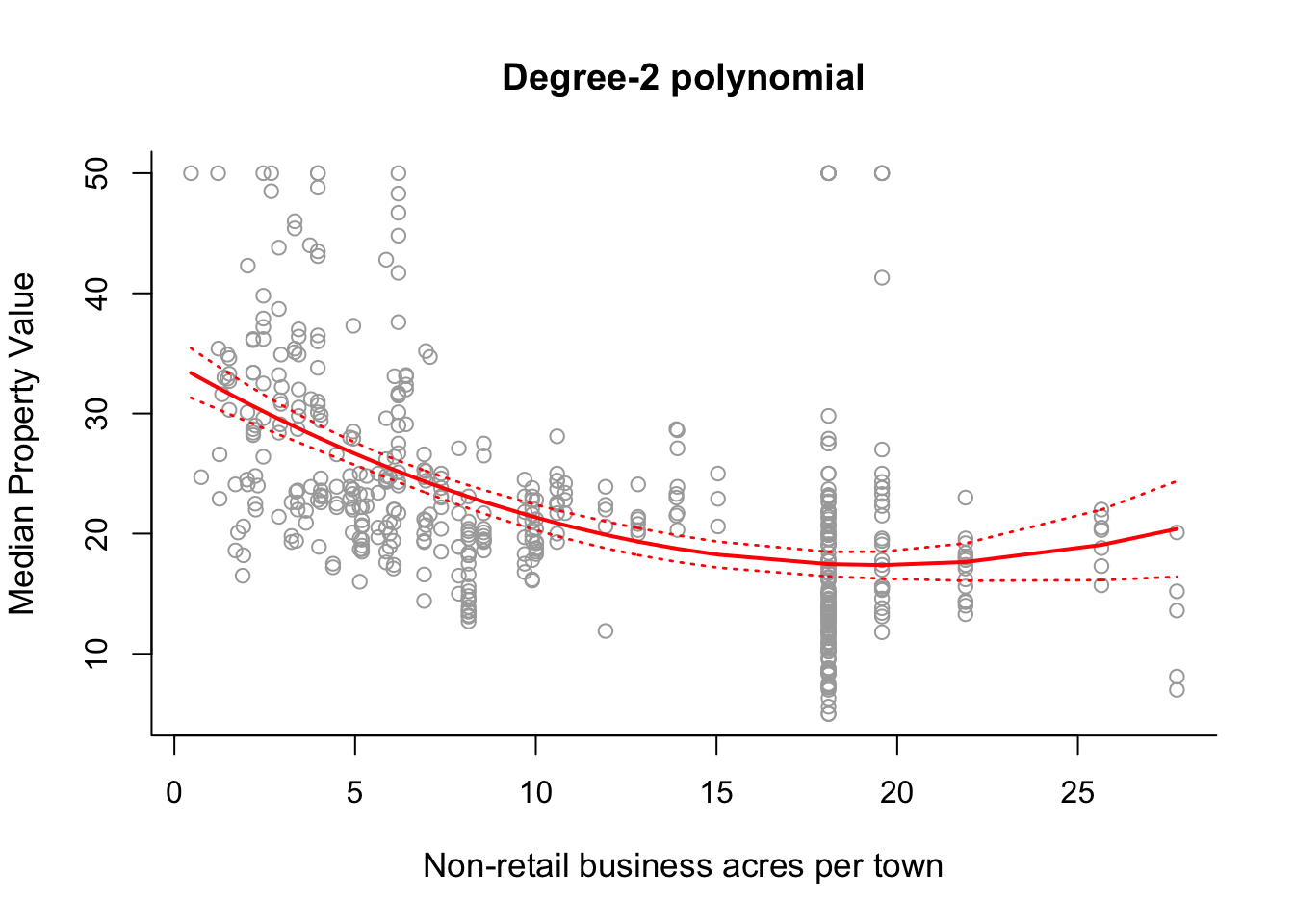
# Repeat the above process for polynomials of degree 3, 4 and 5.
poly3 = lm(y ~ poly(x,  3))
poly4 = lm(y ~ poly(x,  4))
poly5 = lm(y ~ poly(x, 5))

pred3 = predict(poly3, newdata = list(x = sort.x), se = TRUE)
pred4 = predict(poly4, newdata = list(x = sort.x), se = TRUE)
pred5 = predict(poly5, newdata = list(x = sort.x), se = TRUE)

se.bands3 = cbind(pred3$fit + 2*pred3$se.fit, pred3$fit-2*pred3$se.fit)
se.bands4 = cbind(pred4$fit + 2*pred4$se.fit, pred4$fit-2*pred4$se.fit)
se.bands5 = cbind(pred5$fit + 2*pred5$se.fit, pred5$fit-2*pred5$se.fit)

# Display all on one graphics device.
par(mfrow = c(2,2))
# Degree-2
plot(x, y, cex.lab = 1.1, col="darkgrey", xlab = x.lab, ylab = y.lab,
     main = "Degree-2 polynomial", bty = 'l')
lines(sort.x, pred2$fit, lwd = 2, col = "red")
matlines(sort.x, se.bands2, lwd = 2, col = "red", lty = 3)

# Degree-3
plot(x, y, cex.lab = 1.1, col="darkgrey", xlab = x.lab, ylab = y.lab,
     main = "Degree-3 polynomial", bty = 'l')
lines(sort.x, pred3$fit, lwd = 2, col = "darkviolet")
matlines(sort.x, se.bands3, lwd = 2, col = "darkviolet", lty = 3)

# Degree-4
plot(x, y, cex.lab = 1.1, col="darkgrey", xlab = x.lab, ylab = y.lab,
     main = "Degree-4 polynomial", bty = 'l')
lines(sort.x, pred4$fit, lwd = 2, col = "blue")
matlines(sort.x, se.bands4, lwd = 2, col = "blue", lty = 3)

# Degree-5
plot(x, y, cex.lab = 1.1, col="darkgrey", xlab = x.lab, ylab = y.lab,
     main = "Degree-5 polynomial", bty = 'l')
lines(sort.x, pred5$fit, lwd = 2, col = "black")
matlines(sort.x, se.bands5, lwd = 2, col = "black", lty = 3)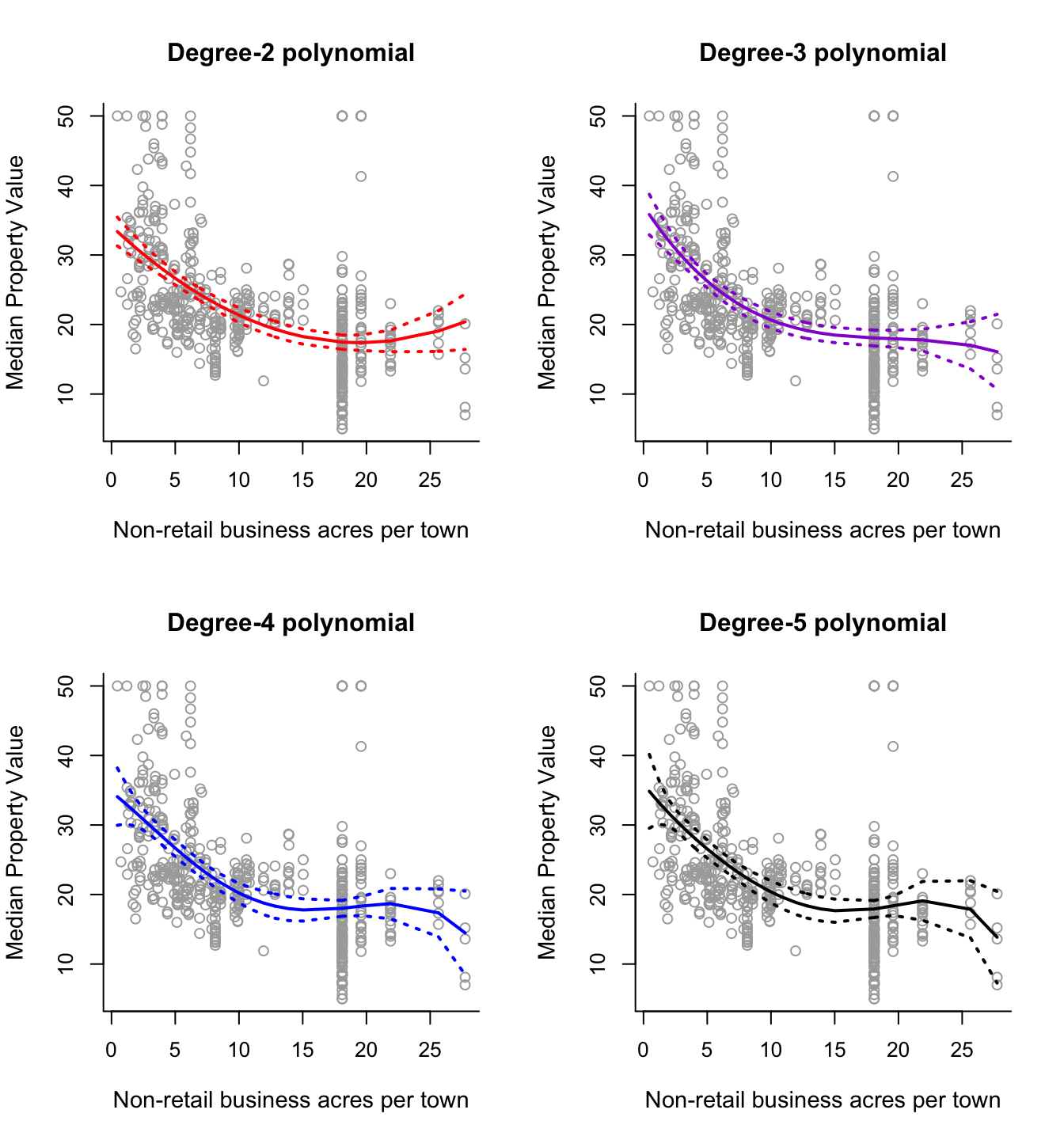
# Lets add in degree 1 and 6 polynomials and perform an ANOVA.
poly1 = lm(y ~ x)
poly6 = lm(y ~ poly(x, 6))
anova(poly1, poly2, poly3, poly4, poly5, poly6)
## Analysis of Variance Table
##
## Model 1: y ~ x
## Model 2: y ~ poly(x, 2)
## Model 3: y ~ poly(x, 3)
## Model 4: y ~ poly(x, 4)
## Model 5: y ~ poly(x, 5)
## Model 6: y ~ poly(x, 6)
## Res.Df RSS Df Sum of Sq F Pr(>F)
## 1 504 32721
## 2 503 31237 1 1483.67 24.1885 1.188e-06 ***
## 3 502 30891 1 346.48 5.6487 0.01784 *
## 4 501 30803 1 87.50 1.4265 0.23291
## 5 500 30790 1 13.15 0.2143 0.64358
## 6 499 30608 1 182.74 2.9793 0.08495 .
## ---
## Signif. codes: 0 '***' 0.001 '**' 0.01 '*' 0.05 '.' 0.1 ' ' 1# anova selects the degree-3 polynomial!
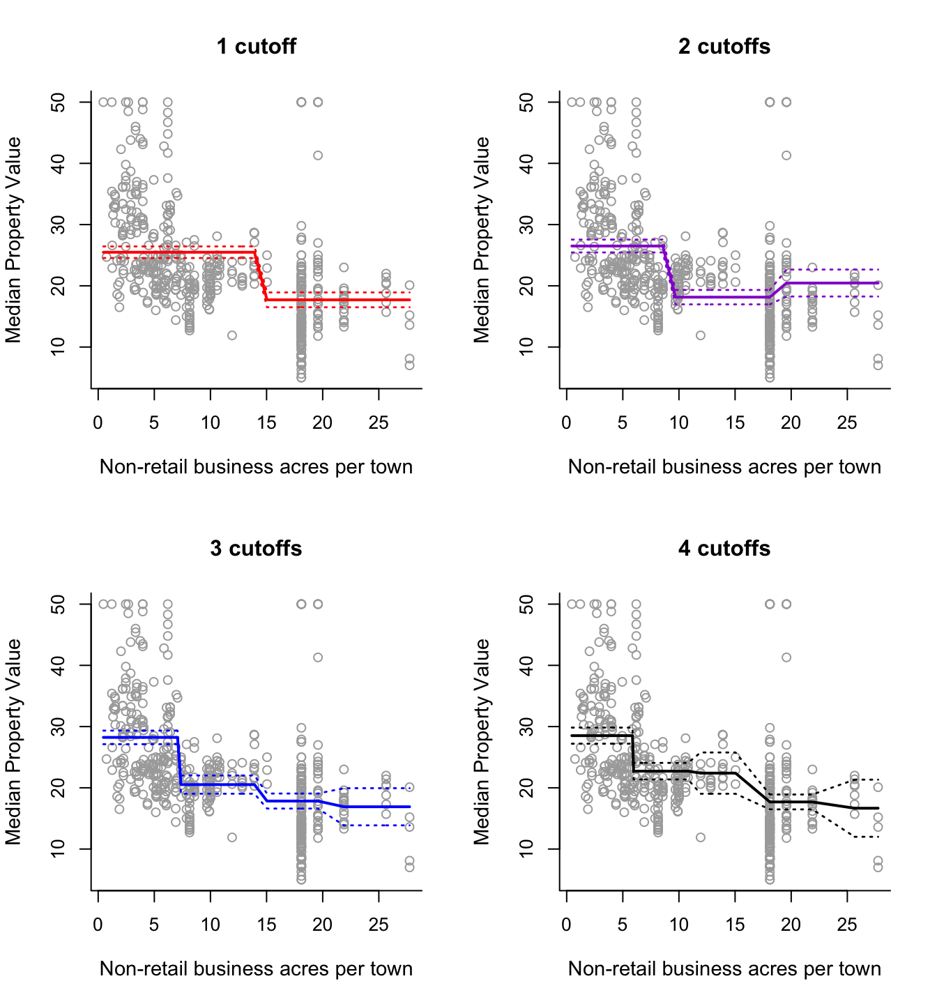
# Step Functions
step2 = lm(y ~ cut(x, 2))
step3 = lm(y ~ cut(x, 3))
step4 = lm(y ~ cut(x, 4))
step5 = lm(y ~ cut(x, 5))
pred2 = predict(step2, newdata = list(x = sort(x)), se = TRUE)
pred3 = predict(step3, newdata = list(x = sort(x)), se = TRUE)
pred4 = predict(step4, newdata = list(x = sort(x)), se = TRUE)
pred5 = predict(step5, newdata = list(x = sort(x)), se = TRUE)
se.bands2 = cbind(pred2$fit + 2*pred2$se.fit, pred2$fit-2*pred2$se.fit)
se.bands3 = cbind(pred3$fit + 2*pred3$se.fit, pred3$fit-2*pred3$se.fit)
se.bands4 = cbind(pred4$fit + 2*pred4$se.fit, pred4$fit-2*pred4$se.fit)
se.bands5 = cbind(pred5$fit + 2*pred5$se.fit, pred5$fit-2*pred5$se.fit)
par(mfrow = c(2,2))
plot(x, y, cex.lab = 1.1, col="darkgrey", xlab = x.lab, ylab = y.lab,
main = "1 cutoff", bty = 'l')
lines(sort(x), pred2$fit, lwd = 2, col = "red")
matlines(sort(x), se.bands2, lwd = 1.4, col = "red", lty = 3)
plot(x, y, cex.lab = 1.1, col="darkgrey", xlab = x.lab, ylab = y.lab,
main = "2 cutoffs", bty = 'l')
lines(sort(x), pred3$fit, lwd = 2, col = "darkviolet")
matlines(sort(x), se.bands3, lwd = 1.4, col = "darkviolet", lty = 3)
plot(x, y, cex.lab = 1.1, col="darkgrey", xlab = x.lab, ylab = y.lab,
main = "3 cutoffs", bty = 'l')
lines(sort(x), pred4$fit, lwd = 2, col = "blue")
matlines(sort(x), se.bands4, lwd = 1.4, col = "blue", lty = 3)
plot(x, y, cex.lab = 1.1, col="darkgrey", xlab = x.lab, ylab = y.lab,
main = "4 cutoffs", bty = 'l')
lines(sort(x), pred5$fit, lwd = 2, col = "black")
matlines(sort(x), se.bands5, lwd = 1.4, col = "black", lty = 3)