Practical 6 Solutions
Make sure to at least finish Question 1 from Practical 5 before continuing with this practical! It might be tempting to skip some stuff if you’re behind, but you may end up more lost\(...\)we will happily answer questions from any previous practical each session.
In Questions 1 and 2, we again analyse the seatpos data from library faraway.
Q1 Splines
In this question, we will again analyse the effects of predictor variable Ht on the response variable hipcenter.
- Load the necessary packages for the dataset and spline functions. Assign the
hipcentervalues to a vectory, and theHtvariable values to a vectorx.
library("MASS")
library("faraway")
library("splines")

y = seatpos$hipcenter
x = seatpos$Ht

# Plot labels for later.
y.lab = 'hip center (mm)'
x.lab = 'Height (bare foot) in cm'- Find the 25th, 50th and 75th percentiles of
x, storing them in a vectorcuts.
summary(x)## Min. 1st Qu. Median Mean 3rd Qu. Max.
## 150.2 163.6 169.5 169.1 175.7 198.4cuts <- summary(x)[c(2,3,5)]- Use a linear spline to model
hipcenteras a function ofHt, putting knots at the 25th, 50th and 75th percentiles ofx.
spline1 = lm(y ~ bs(x, degree = 1, knots = cuts))- Plot the fitted linear spline from part (c) over the data, along with \(\pm2\) standard deviation confidence intervals.
# Sort the values of x from low to high.
sort.x <- sort(x)

# Obtain predictions for the fitted values along with confidence intervals.
pred1 = predict(spline1, newdata = list(x = sort.x), se = TRUE)
se.bands1 = cbind(pred1$fit + 2 * pred1$se.fit, pred1$fit - 2 * pred1$se.fit)

# Plot the fitted linear spline model over the data.
plot(x, y, cex.lab = 1.1, col="darkgrey", xlab = x.lab, ylab = y.lab,
     main = "Linear Spline", bty = 'l')
lines(sort.x, pred1$fit, lwd = 2, col = "red")
matlines(sort.x, se.bands1, lwd = 2, col = "red", lty = 3)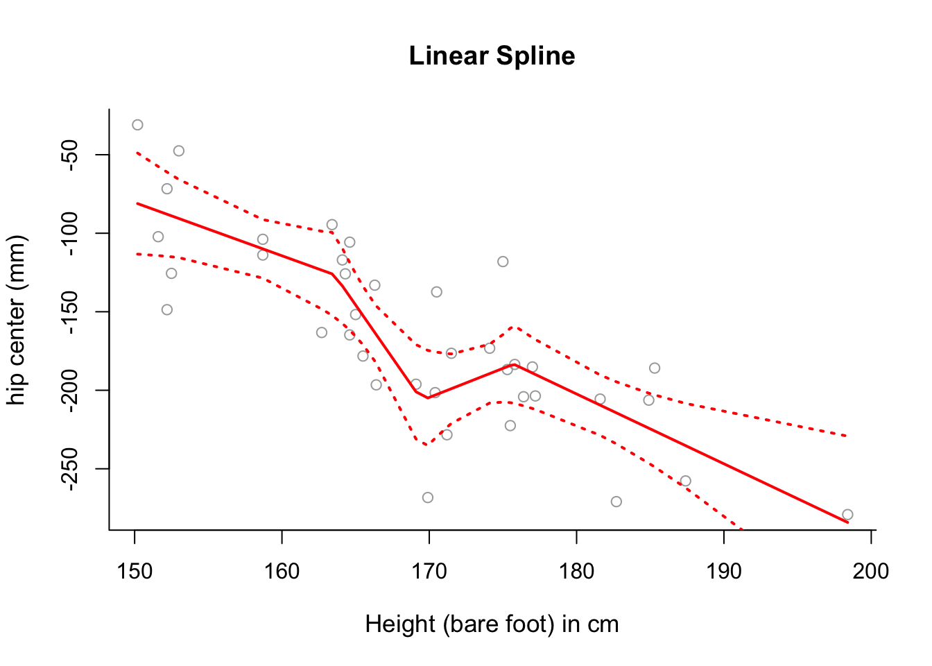
- Use a smoothing spline to model
hipcenteras a function ofHt, selecting \(\lambda\) with cross-validation, and generate a relevant plot. What do you notice?
smooth1 = smooth.spline(x, y, cv = TRUE)## Warning in smooth.spline(x, y, cv = TRUE): cross-validation with non-unique 'x' values
## seems doubtfulplot(x, y, cex.lab = 1.1, col="darkgrey", xlab = x.lab, ylab = y.lab,
main = "Smoothing Spline (3df)", bty = 'l')
lines(smooth1, lwd = 2, col = "brown")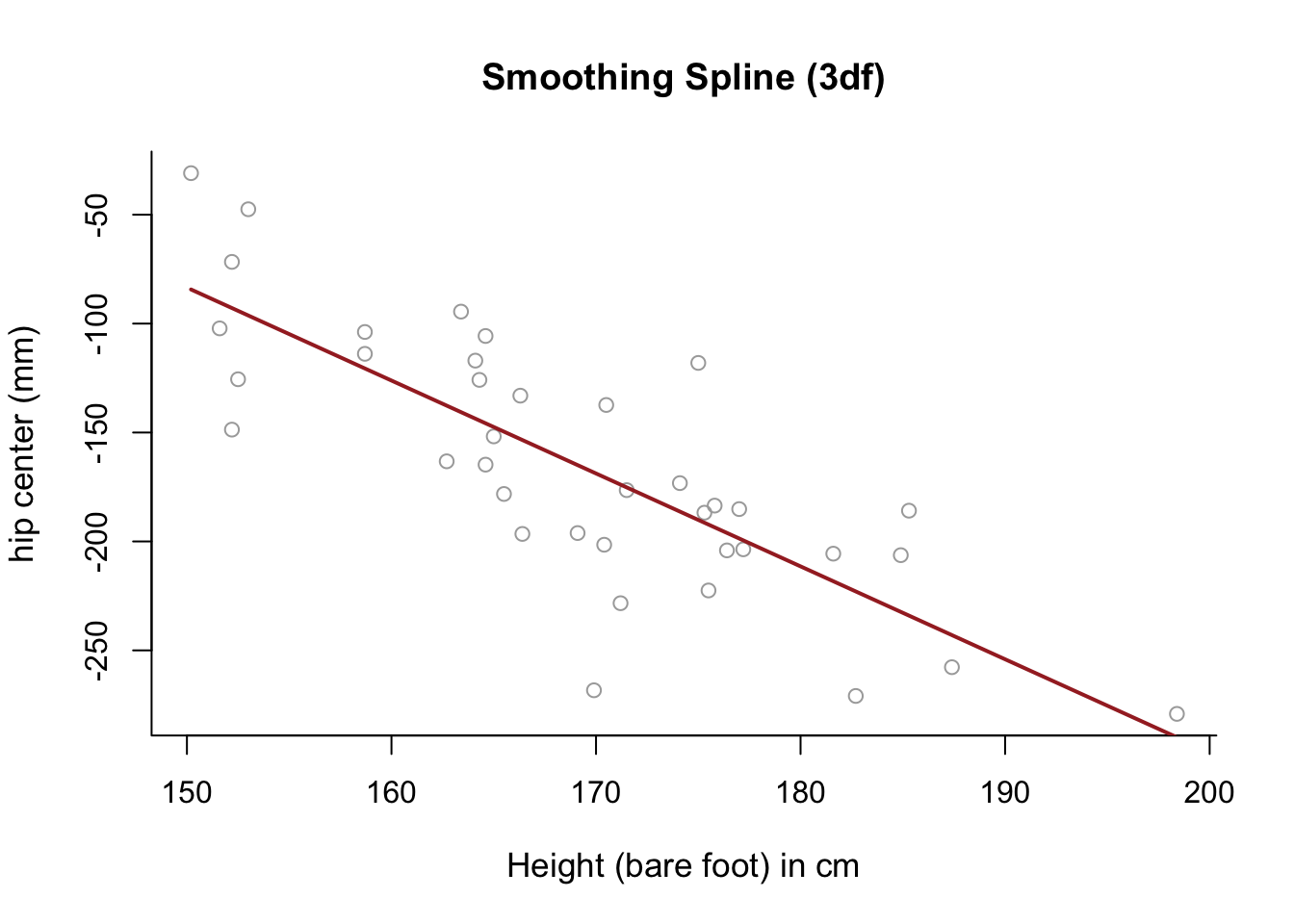
# The fitted model is almost completely linear.Q2 GAMs
- Fit a GAM for
hipcenterthat consists of three terms:
- a natural spline with 5 degrees of freedom for
Age, - a smoothing spline with 3 degrees of freedom for
Thigh, and - a simple linear model term for
Ht.
# Require library gam.
library(gam)

# Fit a GAM.
gam = gam( hipcenter ~ ns( Age, df = 5 ) + s( Thigh, df = 3 ) + Ht,
data = seatpos )- Plot the resulting contributions of each term to the GAM, and compare them with plots of
hipcenteragainst each of the three variablesAge,ThighandHt.
# Plot the contributions.
par( mfrow = c(2,3) )
plot( gam,  se = TRUE, col = "blue" )
# Compare with the following plots.
plot( seatpos$Age, seatpos$hipcenter, pch = 16, col = 2,
      ylab = y.lab, xlab = "Age (years)" )
plot( seatpos$Thigh, seatpos$hipcenter, pch = 16, col = 2,
      ylab = y.lab, xlab = "Thigh length (cm)" )
plot( seatpos$Ht, seatpos$hipcenter, pch = 16, col = 2,
      ylab = y.lab, xlab = "Ht (bare foot) (cm)" )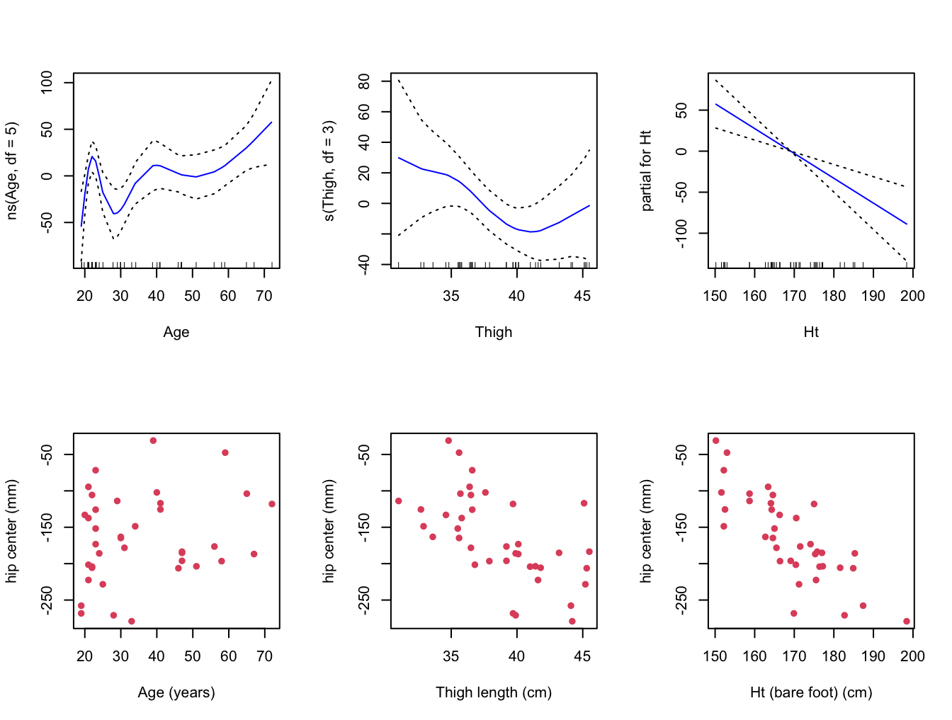
- Does the contribution of each term of the GAM make sense in light of these pair-wise plots. Is the GAM fitting the data well?
# The linear fit of Ht is quite clear.  Perhaps the fits for Age and Thigh
# are less clear, although I think we can see that the curves are fitting
# the data somewhat.
# Perhaps they are overfitting, capturing variation across the predictor
# ranges (in the sample) that isn't really there (in the population).
Q3 Boston Data
- Investigate modelling
medvusing regression, natural and smoothing splines, takingindusas a single predictor.
library(MASS)
library(splines)

y = Boston$medv
x = Boston$indus
y.lab = 'Median Property Value'
x.lab = 'Non-retail business acres per town'

# Use summary on x to find 25th, 50th and 75th percentiles.  We will use
# these for the positions of the knots for regression and natural splines.
summary(x)
## Min. 1st Qu. Median Mean 3rd Qu. Max.
## 0.46 5.19 9.69 11.14 18.10 27.74cuts <- summary(x)[c(2,3,5)]
cuts## 1st Qu. Median 3rd Qu.
## 5.19 9.69 18.10# sort x for later.
sort.x = sort(x)
# Fit a cubic spline
spline.bs = lm(y ~ bs(x, knots = cuts))
pred.bs = predict(spline.bs, newdata = list(x = sort.x), se = TRUE)
se.bands.bs = cbind(pred.bs$fit + 2 * pred.bs$se.fit,
pred.bs$fit - 2 * pred.bs$se.fit)
# Fit a natural cubic spline.
spline.ns = lm(y ~ ns(x, knots = cuts))
pred.ns = predict(spline.ns, newdata = list(x = sort.x), se = TRUE)
se.bands.ns = cbind(pred.ns$fit + 2 * pred.ns$se.fit,
pred.ns$fit - 2 * pred.ns$se.fit)
# Fit a smoothing spline, with 3 effective degrees of freedom.
spline.smooth = smooth.spline(x, y, df = 3)
# Split the plotting device into 3.
par(mfrow = c(1,3))
# Plot the cubic spline.
plot(x, y, cex.lab = 1.1, col="darkgrey", xlab = x.lab, ylab = y.lab,
main = "Cubic Spline", bty = 'l')
lines(sort.x, pred.bs$fit, lwd = 2, col = "red")
matlines(sort.x, se.bands.bs, lwd = 2, col = "red", lty = 3)
# Plot the natural cubic spline.
plot(x, y, cex.lab = 1.1, col="darkgrey", xlab = x.lab, ylab = y.lab,
main = "Natural Cubic Spline", bty = 'l')
lines(sort.x, pred.ns$fit, lwd = 2, col = "darkred")
matlines(sort.x, se.bands.ns, lwd = 2, col = "darkred", lty = 3)
# Plot the smoothing spline.
plot(x, y, cex.lab = 1.1, col="darkgrey", xlab = x.lab, ylab = y.lab,
main = "Smoothing Spline (3 df)", bty = 'l')
lines(spline.smooth, lwd = 2, col = "brown")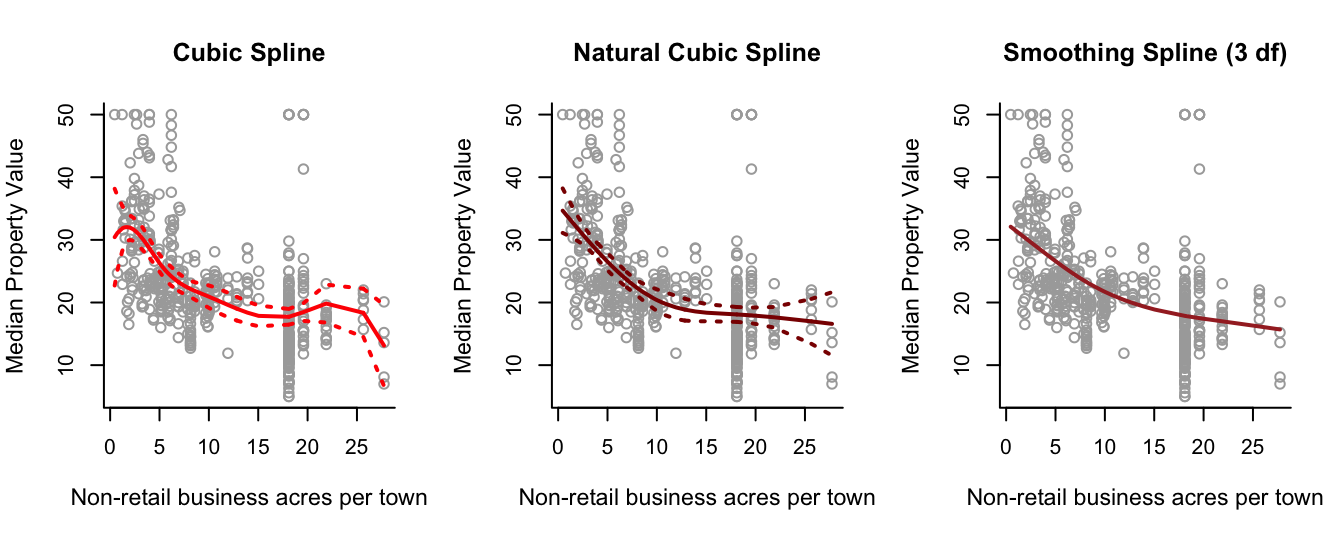
- Choose a set of predictor variables to use in order to fit a GAM for
medv. Feel free to experiment with different modelling options.
# Of course we discussed one possible GAM in practical demonstration
# section of Chapter 10.  We try another one here.

# Let's set chas to be a factor (you may want to make rad a factor as well,
# if used).
Boston1 = Boston
Boston1$chas = factor(Boston1$chas)

# Let's fit a GAM - can you see how each predictor is contributing to
# modelling the response?
gam1 = gam( medv ~ ns( lstat, df = 5 ) + ns( nox, df = 7 ) +
              s( indus, df = 7 ) + poly( age, 5 ) + chas, data = Boston1 )
par(mfrow = c(2,3))
plot(gam1,  se = TRUE, col = "blue")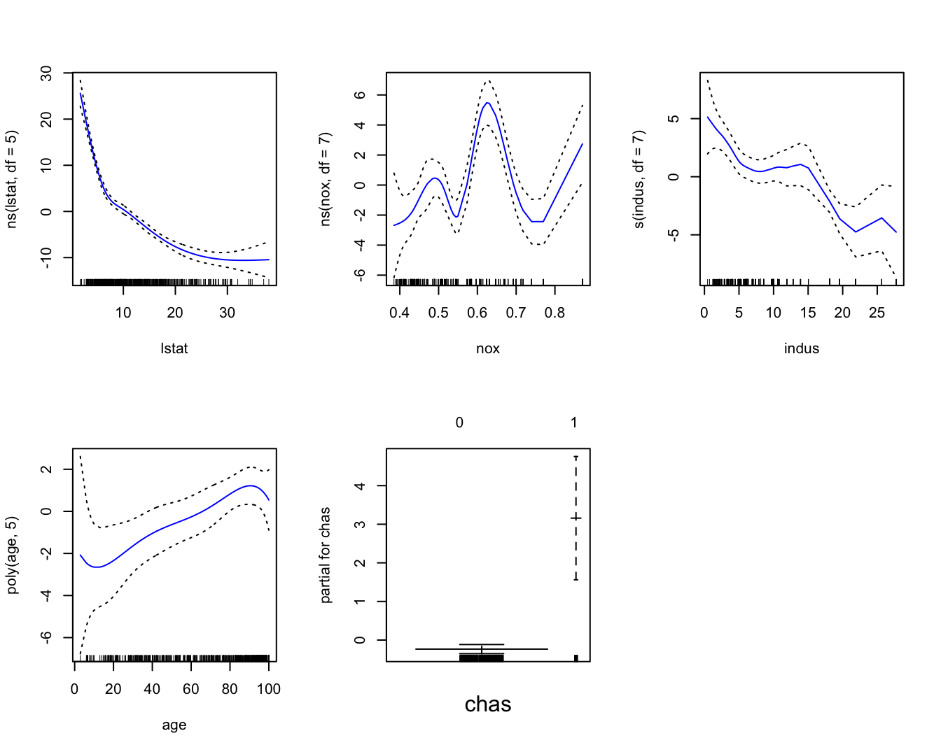
Boyd, S., and L. Vandenberghe. 2009. Convex Optimization. 7th ed. Cambridge: Cambridge University Press.
Faraway, J. J. 2009. Linear Models with r. Edited by F. Dominici, J. J. Faraway, M. Tanner, and J. Zidek. London: CRC press.
Hoerl, Arthur E., and Robert W. Kennard. 1976. “Ridge Regression Iterative Estimation of the Biasing Parameter.” Communications in Statistics - Theory and Methods 5 (1): 77–88. https://doi.org/10.1080/03610927608827333.
Hurwitz, J., and D. Kirsch. 2018. Machine Learning for Dummies. New Jersey: John Wiley & Sons.
James, G., D. Witten, T. Hastie, and R. Tibshirani. 2013. An Introduction to Statistical Learning. Edited by G. Casella, Fienberg S, and I. Olkin. New York: Springer.
Tibshiriani, R. 1996. “Regression Shrinkage and Selection via the Lasso.” Journal of the Royal Statistical Society: Series B (Methodological) 58 (1): 267–88.