Practical 1 Solutions
Note that the questions in all these practicals have multiple possible solutions. Here you will find one that is in line with the course content.
In this first practical we will investigate the dataset fat from the library faraway.
With this data we want to predict body fat (variable brozek) using the other variables available, except for siri (another way of computing body fat), density (it is used in the brozek and siri formulae) and free (it is computed using the brozek formula).
Q1 Data Installation and Initial Manipulation
- If you have not yet done so, install library
faraway.
install.packages("faraway")- Load library
farawayand read the help file on the datasetfat.
library("faraway")
?fat # read the help file for more information about the variables- Look at the top six rows of the dataset
fat. Use relevant commands to find the dimension of the dataframe and the names of the variables.
head(fat) # to look at the top six rows only.## brozek siri density age weight height adipos free neck chest abdom hip thigh knee
## 1 12.6 12.3 1.0708 23 154.25 67.75 23.7 134.9 36.2 93.1 85.2 94.5 59.0 37.3
## 2 6.9 6.1 1.0853 22 173.25 72.25 23.4 161.3 38.5 93.6 83.0 98.7 58.7 37.3
## 3 24.6 25.3 1.0414 22 154.00 66.25 24.7 116.0 34.0 95.8 87.9 99.2 59.6 38.9
## 4 10.9 10.4 1.0751 26 184.75 72.25 24.9 164.7 37.4 101.8 86.4 101.2 60.1 37.3
## 5 27.8 28.7 1.0340 24 184.25 71.25 25.6 133.1 34.4 97.3 100.0 101.9 63.2 42.2
## 6 20.6 20.9 1.0502 24 210.25 74.75 26.5 167.0 39.0 104.5 94.4 107.8 66.0 42.0
## ankle biceps forearm wrist
## 1 21.9 32.0 27.4 17.1
## 2 23.4 30.5 28.9 18.2
## 3 24.0 28.8 25.2 16.6
## 4 22.8 32.4 29.4 18.2
## 5 24.0 32.2 27.7 17.7
## 6 25.6 35.7 30.6 18.8dim(fat) # see what the dimension of the dataframe is. ## [1] 252 18# 252 rows and 18 columns.
names(fat) # the variable names.## [1] "brozek" "siri" "density" "age" "weight" "height" "adipos" "free"
## [9] "neck" "chest" "abdom" "hip" "thigh" "knee" "ankle" "biceps"
## [17] "forearm" "wrist"- Create a new dataframe called
fat1which is equivalent tofat, but with the variablessiri,densityandfreeremoved. Check that the dimension of this new dataframe is correct (that is, the number of rows should be the same as that offatin part (c) and the number of columns should be three less). It is important to get this part correct, as we will use this new dataframefat1throughout the remainder of this practical session.
# Remove variables 2, 3 and 8.
fat1 <- fat[,-c(2,3,8)] # siri is variable 2, density variable 3 and
                        # free variable 8.
dim(fat1) # Check the dimension of the new dataframe.
## [1] 252 15# 252 rows and 15 columns.- Check whether there is any missing data in the (new) dataframe.
sum(is.na(fat1)) # We can just check is.na for the whole ## [1] 0 # dataframe to start with.
# Since the result is zero, there is no missing data.Q2 Exploratory Data Analysis
- Calculate the correlations of
brozekwith respect to the 14 predictor variables.
cor(fat1[,1], fat1[,-1]) ## age weight height adipos neck chest abdom hip
## [1,] 0.2891735 0.6131561 -0.08910641 0.7279942 0.4914889 0.7028852 0.8137062 0.6256999
## thigh knee ankle biceps forearm wrist
## [1,] 0.5612844 0.5077859 0.2667826 0.4930309 0.3632774 0.3475728- Which three predictors have the highest correlations with the response
brozek? Calculate the pair-wise correlation between each of these three predictors. Are they also highly correlated with each other?
# adipos, chest and abdom are the most correlated variables.
# We see that these three predictors exhibit strong correlations
# with the response.  We can check the pair-wise correlations
# between these three variables as well.
cor(fat$adipos, fat$chest)
## [1] 0.9117986cor(fat$adipos, fat$abdom)## [1] 0.9238801cor(fat$chest, fat$abdom)## [1] 0.9158277# These three predictors are all highly correlated with each other as well.- Using the command
pairs(), produce a 4 by 4 frame of scatter plots of the response variable and the three predictors.
pairs( fat[, c("brozek", "adipos", "chest", "abdom")] )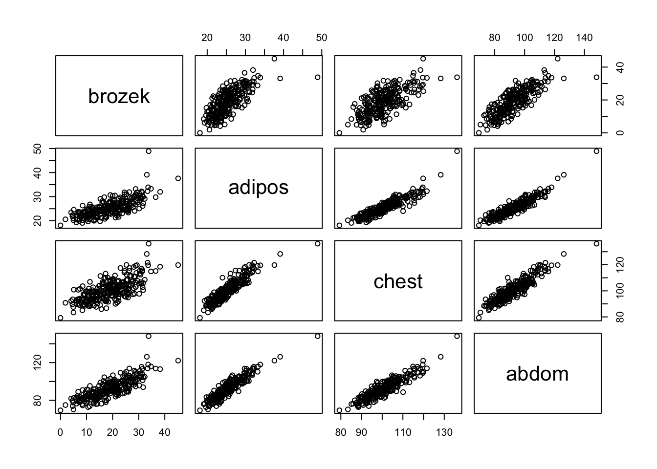
- What does this plot tell us about potential correlations among the three predictors? Does it back up the correlation values obtained in parts (a) and (b)?
# The strong pair-wise positive correlations between the predictors,
# and also between each predictor and the response, is clearly seen
# in the scatter plots.
Q3 Forward Stepwise Regression
- Use
regsubsets()to perform forward stepwise selection, assigning the result to a variable calledfwd. Note that you will need to (install and) load libraryleaps.
library("leaps") # required library for regsubsets() function.
fwd = regsubsets(brozek~., data = fat1, method = 'forward', nvmax = 14)- Look at the summary of the resulting object
fwdand extract the following statistics for the model of each size: RSS, \(R^2\), \(C_p\), BIC and adjusted \(R^2\). Combine them into a single matrix.
results = summary(fwd)
results
## Subset selection object
## Call: regsubsets.formula(brozek ~ ., data = fat1, method = "forward",
## nvmax = 14)
## 14 Variables (and intercept)
## Forced in Forced out
## age FALSE FALSE
## weight FALSE FALSE
## height FALSE FALSE
## adipos FALSE FALSE
## neck FALSE FALSE
## chest FALSE FALSE
## abdom FALSE FALSE
## hip FALSE FALSE
## thigh FALSE FALSE
## knee FALSE FALSE
## ankle FALSE FALSE
## biceps FALSE FALSE
## forearm FALSE FALSE
## wrist FALSE FALSE
## 1 subsets of each size up to 14
## Selection Algorithm: forward
## age weight height adipos neck chest abdom hip thigh knee ankle biceps forearm
## 1 ( 1 ) " " " " " " " " " " " " "*" " " " " " " " " " " " "
## 2 ( 1 ) " " "*" " " " " " " " " "*" " " " " " " " " " " " "
## 3 ( 1 ) " " "*" " " " " " " " " "*" " " " " " " " " " " " "
## 4 ( 1 ) " " "*" " " " " " " " " "*" " " " " " " " " " " "*"
## 5 ( 1 ) " " "*" " " " " "*" " " "*" " " " " " " " " " " "*"
## 6 ( 1 ) "*" "*" " " " " "*" " " "*" " " " " " " " " " " "*"
## 7 ( 1 ) "*" "*" " " " " "*" " " "*" " " "*" " " " " " " "*"
## 8 ( 1 ) "*" "*" " " " " "*" " " "*" "*" "*" " " " " " " "*"
## 9 ( 1 ) "*" "*" " " " " "*" " " "*" "*" "*" " " " " "*" "*"
## 10 ( 1 ) "*" "*" " " " " "*" " " "*" "*" "*" " " "*" "*" "*"
## 11 ( 1 ) "*" "*" "*" " " "*" " " "*" "*" "*" " " "*" "*" "*"
## 12 ( 1 ) "*" "*" "*" " " "*" "*" "*" "*" "*" " " "*" "*" "*"
## 13 ( 1 ) "*" "*" "*" "*" "*" "*" "*" "*" "*" " " "*" "*" "*"
## 14 ( 1 ) "*" "*" "*" "*" "*" "*" "*" "*" "*" "*" "*" "*" "*"
## wrist
## 1 ( 1 ) " "
## 2 ( 1 ) " "
## 3 ( 1 ) "*"
## 4 ( 1 ) "*"
## 5 ( 1 ) "*"
## 6 ( 1 ) "*"
## 7 ( 1 ) "*"
## 8 ( 1 ) "*"
## 9 ( 1 ) "*"
## 10 ( 1 ) "*"
## 11 ( 1 ) "*"
## 12 ( 1 ) "*"
## 13 ( 1 ) "*"
## 14 ( 1 ) "*"RSS = results$rss
r2 = results$rsq
Cp = results$cp
BIC = results$bic
Adj_r2 = results$adjr2
# Combine the calculated criteria values above into a single matrix.
criteria_values <- cbind(RSS, r2, Cp, BIC, Adj_r2)
criteria_values## RSS r2 Cp BIC Adj_r2
## [1,] 5094.931 0.6621178 71.075501 -262.3758 0.6607663
## [2,] 4241.328 0.7187265 19.617727 -303.0555 0.7164672
## [3,] 4108.183 0.7275563 13.279341 -305.5638 0.7242606
## [4,] 3994.311 0.7351080 8.147986 -307.1180 0.7308182
## [5,] 3950.628 0.7380049 7.412297 -304.3597 0.7326798
## [6,] 3913.377 0.7404753 7.079431 -301.2177 0.7341196
## [7,] 3853.214 0.7444651 5.311670 -299.5925 0.7371342
## [8,] 3819.985 0.7466688 5.230664 -296.2456 0.7383287
## [9,] 3805.075 0.7476576 6.296894 -291.7018 0.7382730
## [10,] 3793.873 0.7484005 7.595324 -286.9153 0.7379607
## [11,] 3786.200 0.7489093 9.114827 -281.8960 0.7374010
## [12,] 3785.179 0.7489771 11.050872 -276.4346 0.7363734
## [13,] 3784.367 0.7490309 13.000019 -270.9592 0.7353225
## [14,] 3784.367 0.7490309 15.000000 -265.4298 0.7342058- How many predictors are included in the models with i) minimum \(C_p\), ii) minimum BIC, and iii) maximum adjusted \(R^2\)? Which predictors are included in each case?
which.min(Cp) # i) 8## [1] 8which.min(BIC) # ii) 4## [1] 4which.max(Adj_r2) # iii) 8## [1] 8coef(fwd, 4)## (Intercept) weight abdom forearm wrist
## -31.2967858 -0.1255654 0.9213725 0.4463824 -1.3917662# Looking at the summary above, the model with 4 predictors (minimum BIC)
# includes the predictors weight, abdom, forearm and wrist.
coef(fwd, 8)## (Intercept) age weight neck abdom hip
## -20.06213373 0.05921577 -0.08413521 -0.43189267 0.87720667 -0.18641032
## thigh forearm wrist
## 0.28644340 0.48254563 -1.40486912# The model with 8 predictors (minimum Cp and maximum adjusted R-squared)
# includes additionally the predictors age, neck, hip and thigh.- In a single plotting window, generate the following three plots, showing the relationship between the two variables as lines (as seen in the practical demonstration 2.4): i) \(C_p\) against number of predictors, ii) BIC against number of predictors, and iii) adjusted \(R^2\) against number of predictors. Make sure to add relevant labels to the plots. Highlight the optimal model appropriately on each plot using a big red point.
par(mfrow = c(1, 3))
plot(Cp, xlab = "Number of Predictors", ylab = "Cp", type = 'l', lwd = 2)
points(8, Cp[8], col = "red", cex = 2, pch = 8, lwd = 2)
plot(BIC, xlab = "Number of Predictors", ylab = "BIC", type = 'l', lwd = 2)
points(4, BIC[4], col = "red", cex = 2, pch = 8, lwd = 2)
plot(Adj_r2, xlab = "Number of Predictors", ylab = "Adjusted RSq",
     type = "l", lwd = 2)
points(8, Adj_r2[8],  col = "red", cex = 2, pch = 8, lwd = 2)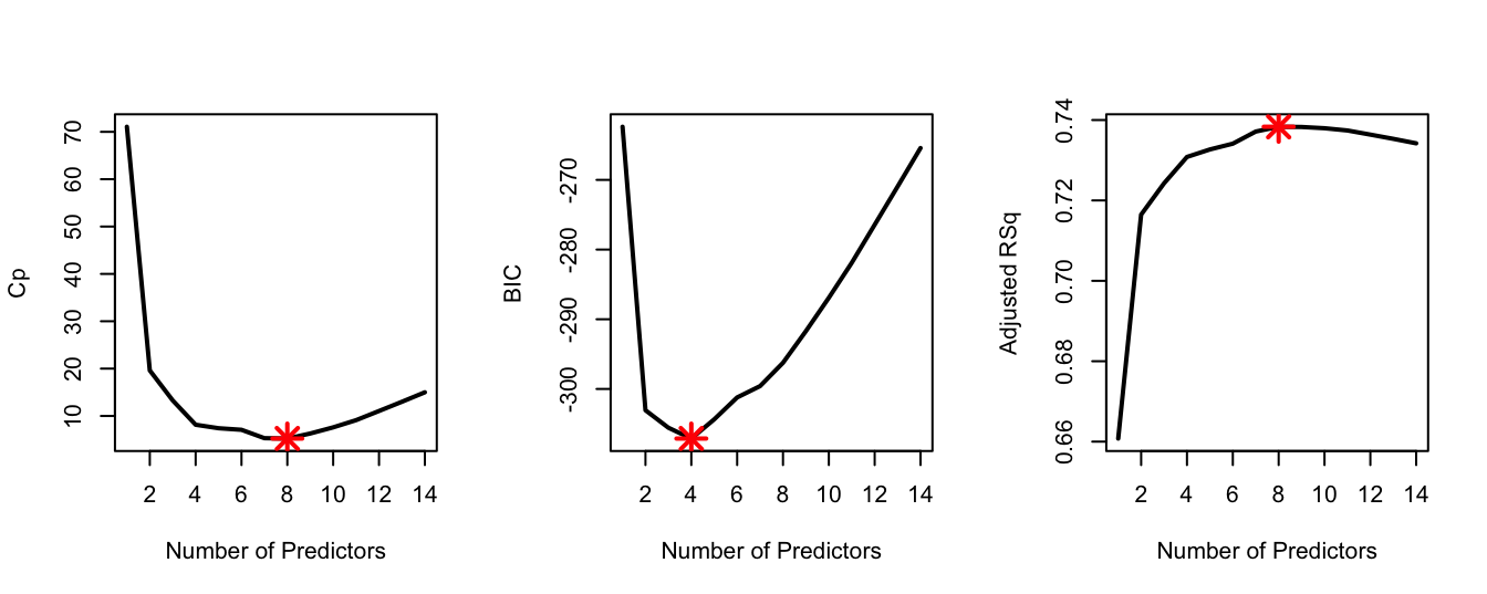
- Use the special
plot()function forregsubsetsto visualise the models obtained by \(C_p\).
plot(fwd, scale = "Cp")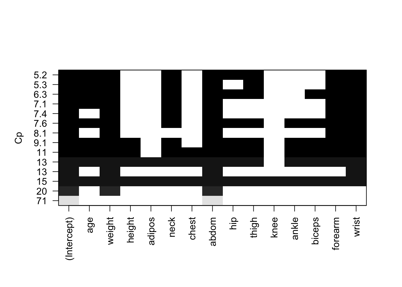
Q4 Best Subset and Backward Selection
Do the best models (as determined by \(C_p\), BIC and adjusted-\(R^2\)) from best subset and backward stepwise selections have the same number of predictors? If yes, are the predictors the same as those from forward selection? Hint: if it is not obvious how to perform backward selection type ?regsubsets and see information about argument method.
best = regsubsets(brozek~., data = fat1, nvmax = 14)
bwd = regsubsets(brozek~., data = fat1, method = 'backward', nvmax = 14)

which.min(summary(best)$cp)
## [1] 8which.min(summary(best)$bic)## [1] 4which.max(summary(best)$adjr2)## [1] 8which.min(summary(bwd)$cp)## [1] 8which.min(summary(bwd)$bic)## [1] 4which.max(summary(bwd)$adjr2)## [1] 8# Yes, the three optimal models (under each of the criteria Cp, BIC and
# adj-R-squared) for each of forward stepwise, backward stepwise and
# best subset selections all have the same number of predictors.
# Cp
coef(fwd,8) ## (Intercept) age weight neck abdom hip
## -20.06213373 0.05921577 -0.08413521 -0.43189267 0.87720667 -0.18641032
## thigh forearm wrist
## 0.28644340 0.48254563 -1.40486912coef(best,8) ## (Intercept) age weight neck abdom hip
## -20.06213373 0.05921577 -0.08413521 -0.43189267 0.87720667 -0.18641032
## thigh forearm wrist
## 0.28644340 0.48254563 -1.40486912coef(bwd,8)## (Intercept) age weight neck abdom hip
## -20.06213373 0.05921577 -0.08413521 -0.43189267 0.87720667 -0.18641032
## thigh forearm wrist
## 0.28644340 0.48254563 -1.40486912# BIC
coef(fwd,4) ## (Intercept) weight abdom forearm wrist
## -31.2967858 -0.1255654 0.9213725 0.4463824 -1.3917662coef(best,4) ## (Intercept) weight abdom forearm wrist
## -31.2967858 -0.1255654 0.9213725 0.4463824 -1.3917662coef(bwd,4)## (Intercept) weight abdom forearm wrist
## -31.2967858 -0.1255654 0.9213725 0.4463824 -1.3917662# In addition, the predictors are also the same.
# Note that comparison of the models under R-squared is as for
# Cp as this criterion also suggested the model with 8 predictors.