4.1 Supervised Learning

Supervised learning involves predicting an output variable given a set of input variables.

In the supervised learning setting, we typically have access to a set of p features $X_1, X_2, \dots, X_p$ , measured on $n$ observations, and a response $Y$ also measured on those same n observations.

The goal is then to predict $Y$ using $X_1, X_2, \dots, X_p$ .

4.1.1 Regression

Here, we assume that $Y$ is a numeric variable. The goal is the predict the value of $Y_i$ for a given input of $X_{i1},X_{i2},...,X_{ik}$

Linear Regression

This is taught in your Stat 136, where the quantitative variable $Y$ is a linear function of the predictors $X_1, X_2,...,X_k$

Advertising <- read.csv("advertising.csv")
Advertising

ABCDEFGHIJ0123456789

id <int>	tv <dbl>	radio <dbl>	newspaper <dbl>	sales <dbl>
1	230.1	37.8	69.2	22.1
2	44.5	39.3	45.1	10.4
3	17.2	45.9	69.3	9.3
4	151.5	41.3	58.5	18.5
5	180.8	10.8	58.4	12.9
6	8.7	48.9	75.0	7.2
7	57.5	32.8	23.5	11.8
8	120.2	19.6	11.6	13.2
9	8.6	2.1	1.0	4.8
10	199.8	2.6	21.2	10.6

Using this dataset, we want to fit this to the model:

$sales = \beta_0 +\beta_1 \text{TV} +\beta_2\text{radio} +\beta_3\text{newspaper} +\varepsilon$

When predicting the value of sales given the value of advertising expenditure on TV, radio, and newspaper, the coefficients $\beta_0,\beta_1,\beta_2,\beta_3$ must be estimated, to make predictions using the formula:

$\hat{y} = \hat{\beta_0} +\hat{\beta_1}x_1 + \hat{\beta_2}x_2 + \hat{\beta_3}x_3$

For this example, let us use the first 100 observations for fitting the model.

Adv_1 <- Advertising[1:100,]
adv <- lm(sales ~ tv + radio +newspaper, data=Adv_1)
summary(adv)

## 
## Call:
## lm(formula = sales ~ tv + radio + newspaper, data = Adv_1)
## 
## Residuals:
##     Min      1Q  Median      3Q     Max 
## -5.1389 -0.7700  0.1999  1.0781  2.7124 
## 
## Coefficients:
##              Estimate Std. Error t value Pr(>|t|)    
## (Intercept)  3.349785   0.426742   7.850  5.9e-12 ***
## tv           0.045513   0.001892  24.061  < 2e-16 ***
## radio        0.192088   0.012468  15.407  < 2e-16 ***
## newspaper   -0.010666   0.008235  -1.295    0.198    
## ---
## Signif. codes:  0 '***' 0.001 '**' 0.01 '*' 0.05 '.' 0.1 ' ' 1
## 
## Residual standard error: 1.556 on 96 degrees of freedom
## Multiple R-squared:  0.911,  Adjusted R-squared:  0.9083 
## F-statistic: 327.7 on 3 and 96 DF,  p-value: < 2.2e-16

Now, we use the model adv to predict sales of the last 100 observations.

Adv_2 <- Advertising[101:200,]

sales_predicted <- predict(adv,Adv_2)

plot(Adv_2$sales, sales_predicted)

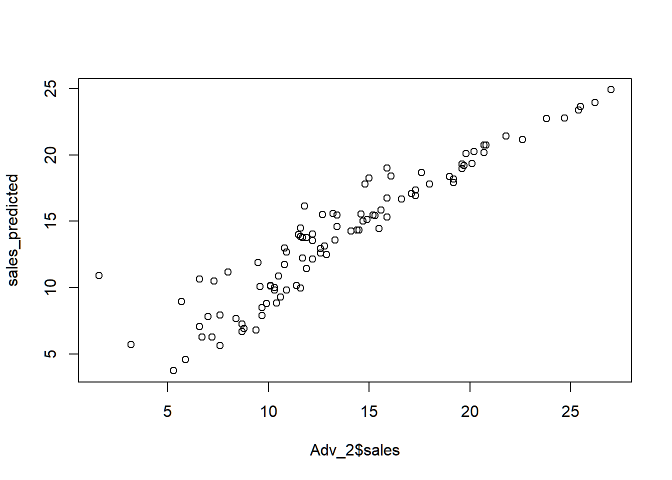
From this graph, the predicted sales is almost the same as the actual sales, indicating a good model for predicting sales.

Polynomial Regression

Historically, the standard way to extend linear regression to settings in which the relationship between the predictors and the response is non-linear has been to replace the standard linear model

$y_i=\beta_0 + \beta_1x_i +\varepsilon_i$

with a polynomial function:

$y_i = \beta_0 + \beta_1x_i+\beta_2x_i^2+ \beta_3x_i^3+\cdots+\beta_dx_i^d+\varepsilon_i$

This approach is known as polynomial regression. For large enough degree $d$ , a polynomial regression allows us to produce an extremely non-linear curve.

Let us explore the mtcars dataset, creating a model that predicts mpg using hp. In the following graph, the relationship of the two variables do not seem linear.

mtcars_plot <- ggplot(mtcars, aes(x = hp, y = mpg)) +
        geom_point()
mtcars_plot

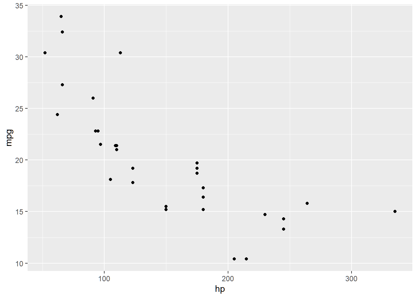
We fit the data on the following model:

$mpg = \beta_0 + \beta_1 hp+\beta_2(hp)^2+\varepsilon$

model_poly <- lm(mpg ~ hp + I(hp^2), data = mtcars)
summary(model_poly)

## 
## Call:
## lm(formula = mpg ~ hp + I(hp^2), data = mtcars)
## 
## Residuals:
##     Min      1Q  Median      3Q     Max 
## -4.5512 -1.6027 -0.6977  1.5509  8.7213 
## 
## Coefficients:
##               Estimate Std. Error t value Pr(>|t|)    
## (Intercept)  4.041e+01  2.741e+00  14.744 5.23e-15 ***
## hp          -2.133e-01  3.488e-02  -6.115 1.16e-06 ***
## I(hp^2)      4.208e-04  9.844e-05   4.275 0.000189 ***
## ---
## Signif. codes:  0 '***' 0.001 '**' 0.01 '*' 0.05 '.' 0.1 ' ' 1
## 
## Residual standard error: 3.077 on 29 degrees of freedom
## Multiple R-squared:  0.7561, Adjusted R-squared:  0.7393 
## F-statistic: 44.95 on 2 and 29 DF,  p-value: 1.301e-09

mtcars_f <- function(x){
    model_poly$coefficients[1] +
        model_poly$coefficients[2] * x +
        model_poly$coefficients[3] * x^2
}
mtcars_plot +
    geom_function(fun = mtcars_f)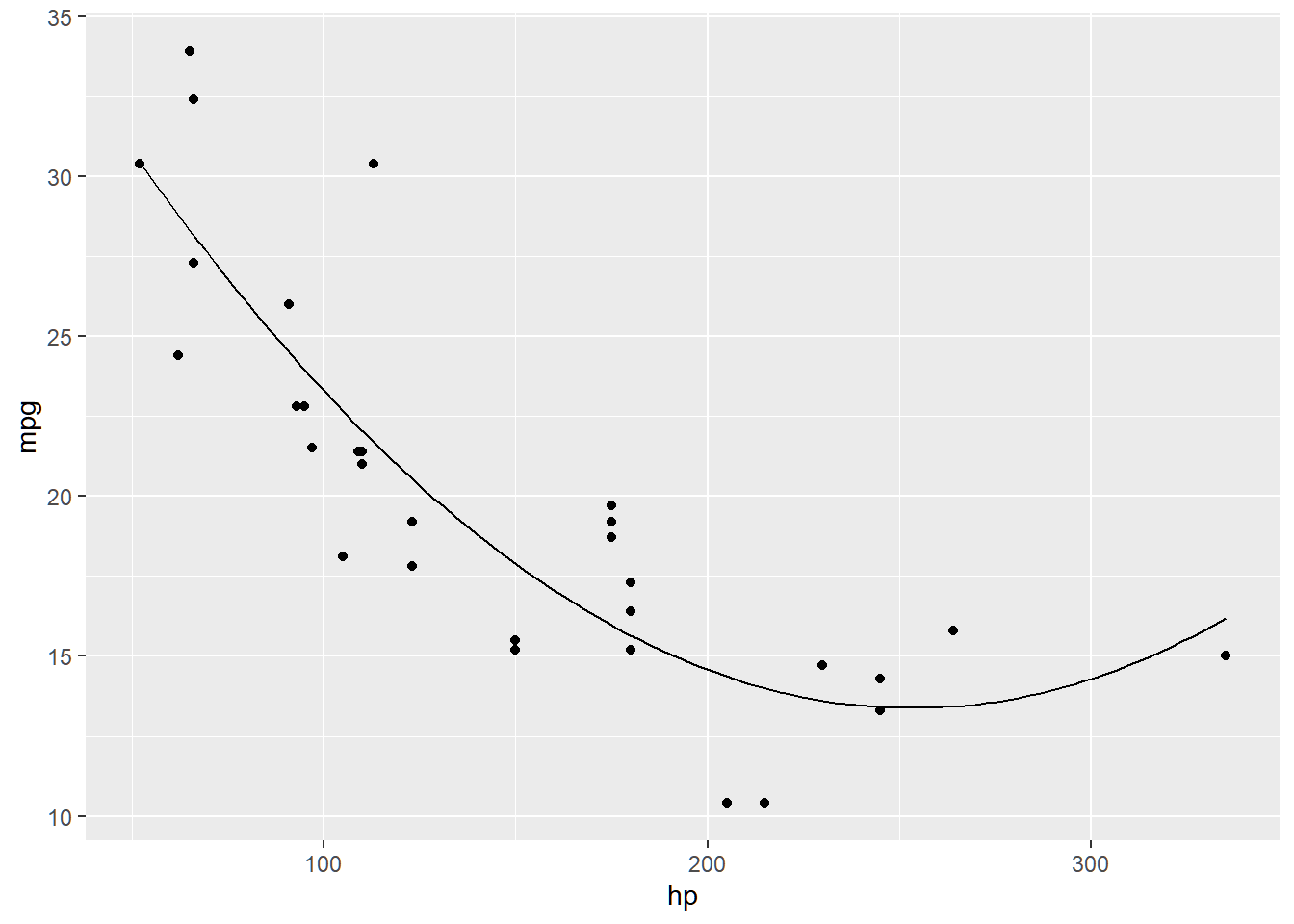

Same with linear regression, careful when predicting value of $Y$ using values of $X$ that is outside the range of the dataset. For this example, you cannot extrapolate for a predicted value of $mpg$ for $hp>335$ .

Smoothing Spline

In ﬁtting a smooth curve to a set of data, what we really want to do is ﬁnd some function, say $g(x)$ , that ﬁts the observed data well. That is, we want $SSE=\sum_{i=1}^n(y_i-g(x_i))^2$ to be small.

However, there is a problem with this approach. If we do not put constraints on $g(x_i)$ , then we can make $SSE$ zero by simply selecting a function $g$ that interpolates all points (i.e. $g(x)=y$ ).

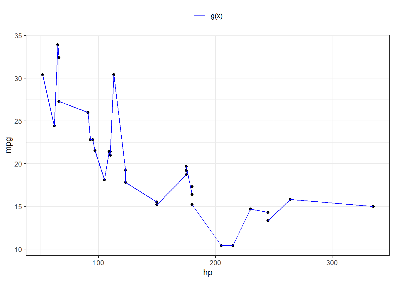
Such a function would woefully overﬁt the data. What we really want is a function $g$ that makes RSS small, but that is also smooth.

How might we ensure that $g$ is smooth? There are a number of ways to do this. A natural approach is to ﬁnd the function $g$ that minimizes

$\begin{equation} \sum_{i=1}^n(y_i-g(x_i))^2 + \lambda \int g''(t)^2dt \tag{4.1} \end{equation}$

where $\lambda$ is a nonnegative tuning parameter. The function $g$ that minimizes the equation above is called a smoothing spline.

(4.1) takes the “Loss+Penalty” formulation. The term $\sum\_{i=1}^n(y_i-g(x_i))^2$ is a loss function, and the term $\lambda \int g''(t)\^2dt$ is a penalty term that penalizes the variability in $g$ .

## `geom_smooth()` using method
## = 'loess' and formula = 'y ~
## x'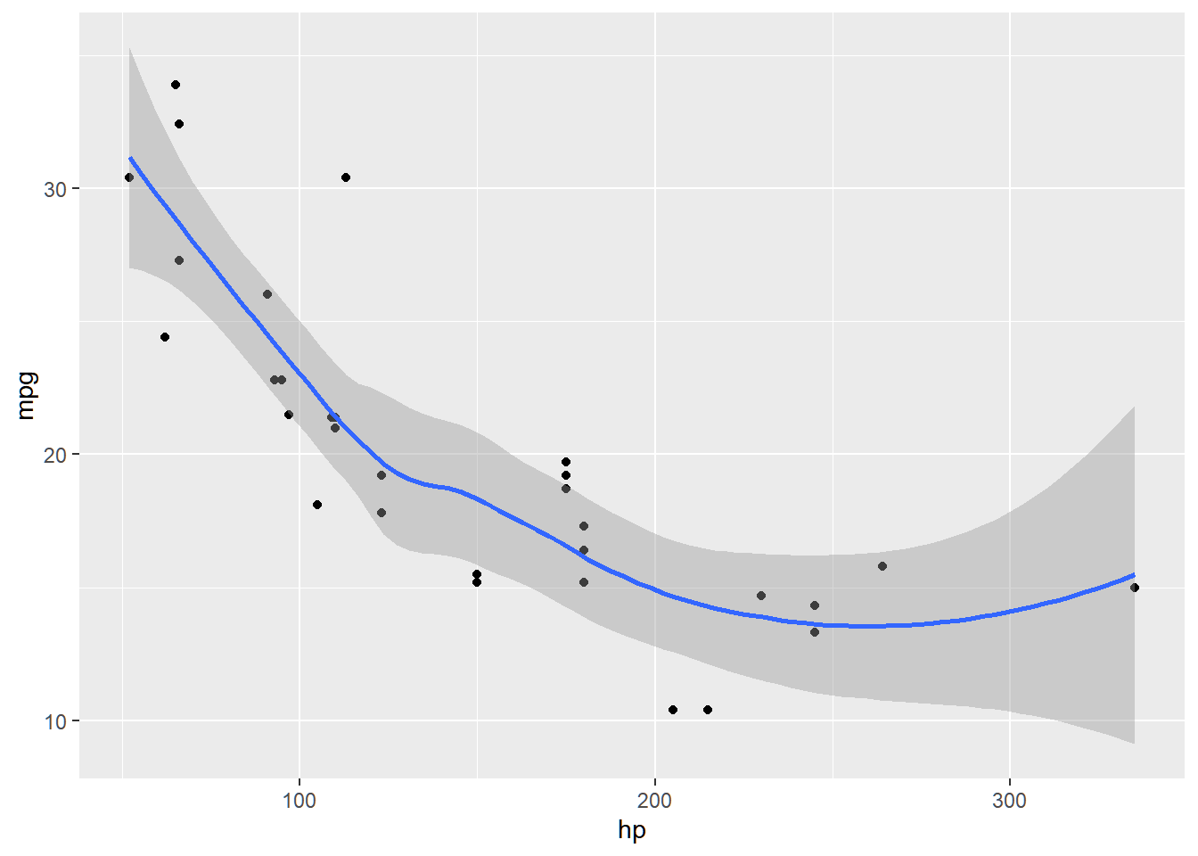

In order to ﬁt regression splines in R, we use the splines library.

library(splines)

In this example, we also use the Wage data from ISLR package.

#Wage

Fitting wage toageusing a smooth spline is simple. We use thesmooth.spline()` function.

#fit <- smooth.spline(Wage$age, Wage$wage, df=16)
#fit

4.1.2 Classification

Classification is a supervised learning task where the objective is to assign labels to instances based on their features. Typical applications include fraud detection, medical diagnosis, and image recognition.

Unlike regression, where the output is continuous, classification problems require that the dependent variable $Y$ is a categorical variable.

Logistic Regression

Logistic Regression is one of the simplest yet powerful classification algorithms. Despite its name, it is used for classification tasks, not regression.

Theory

Logistic Regression models the probability that an instance belongs to a particular class. For binary classification, it estimates the probability of the positive class using the logistic (sigmoid) function:

$P(Y=1|\textbf{X})= \frac{\exp{(\beta_0+\beta_1 X_1 + \cdots+\beta_kX_k)}}{1+\exp{(\beta_0+\beta_1 X_1 + \cdots+\beta_kX_k)}}$

The model parameters $\beta$ may be estimated using Maximum Likelihood Estimation.

Advantages

Easy to implement and interpret.
Works well when the relationship between features and the log-odds of the target is linear.

Disadvantages

Struggles with complex relationships.
Assumes independence of features.

# Fit a logistic regression model
model <- glm(am ~ hp + wt, data = mtcars, family = binomial)
# Summary of the model
summary(model)

## 
## Call:
## glm(formula = am ~ hp + wt, family = binomial, data = mtcars)
## 
## Coefficients:
##             Estimate Std. Error z value Pr(>|z|)   
## (Intercept) 18.86630    7.44356   2.535  0.01126 * 
## hp           0.03626    0.01773   2.044  0.04091 * 
## wt          -8.08348    3.06868  -2.634  0.00843 **
## ---
## Signif. codes:  0 '***' 0.001 '**' 0.01 '*' 0.05 '.' 0.1 ' ' 1
## 
## (Dispersion parameter for binomial family taken to be 1)
## 
##     Null deviance: 43.230  on 31  degrees of freedom
## Residual deviance: 10.059  on 29  degrees of freedom
## AIC: 16.059
## 
## Number of Fisher Scoring iterations: 8

Naïve Bayes Classifier

Support Vector Machine

Support vector machine (SVM) is an approach for classiﬁcation that was developed in the computer science community in the 1990s and that has grown in popularity since then. SVMs have been shown to perform well in a variety of settings, and are often considered one of the best “out of the box” classiﬁers.

The support vector machine is a generalization of maximal margin classiﬁer and support vector classifier.

People often loosely refer to the maximal margin classiﬁer, the support vector classiﬁer, and the support vector machine as “support vector machines”. To avoid confusion, we will carefully distinguish between these three notions in this chapter.

Maximal Margin Classifier

In this section, we deﬁne a hyperplane and introduce the concept of an optimal separating hyperplane.

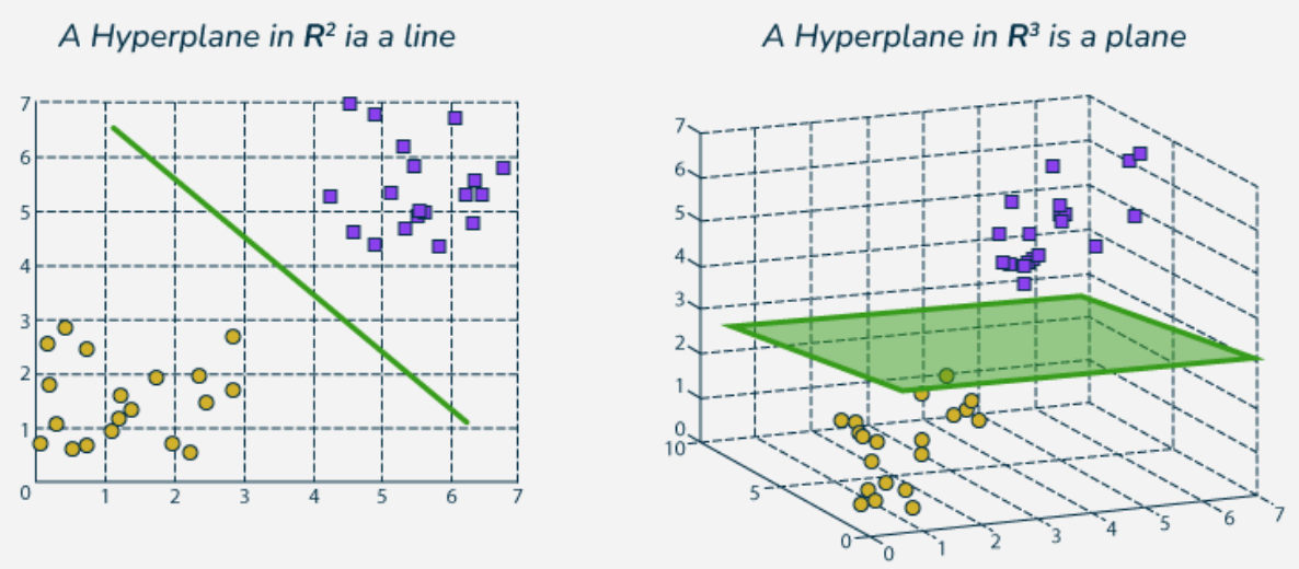
Definition 4.1 In a $p$ -dimensional space, a hyperplane is a ﬂat affine subspace of hyperplane dimension $p − 1$

For instance, in two dimensions, a hyperplane is 1 dimensional, that is, a line. In three dimensions, a hyperplane is 2 dimensional, that is, a plane.

Mathematically, the hyperplane in the $p$ -dimensional setting is defined by the equation

$\begin{equation} \beta_0 + \beta_1X_1 +\beta_2X_2+\cdots+\beta_pX_p = 0 \tag{4.2} \end{equation}$

If a point $X=(X_1,X_2,...,X_p)'$ satisfies the equation (4.2) above, then $X$ lies on the hyperplane.
If $\beta_0 + \beta_1X_1 +\beta_2X_2+\cdots+\beta_pX_p > 0$ , then $X$ is on one side of the hyperplane.
On the other hand, if $\beta_0 + \beta_1X_1 +\beta_2X_2+\cdots+\beta_pX_p < 0$ , then $X$ is on the other side of the hyperplane.

So we can think of the hyperplane as dividing p-dimensional space into two halves. One can easily determine on which side of the hyperplane a point lies by simply calculating the sign of the left hand side of the equation (4.2).

When classifying data using hyperplanes, there will be an infinite number of such hyperplanes. A natural choice is the maximal margin hyperplane.

Definition 4.2 The Maximal Margin Hyperplane (also known as the optimal separating hyperplane) is the separating hyperplane that is farthest from the training observations.

That is, we can compute the (perpendicular) distance from each training observation to a given separating hyperplane

Definition 4.3 The smallest such distance is the minimal distance from the observations to the hyperplane, and is known as the margin.

Definition 4.4 The datapoints that are closest to the optimal separating hyperplane is called the support vector

The support vectors “support” the maximal margin hyperplane in the sense that if these points were moved slightly, then the maximal margin hyperplane would move as well.

Interestingly, the maximal margin hyperplane depends directly on the support vectors, but not on the other observations: a movement to any of the other observations would not aﬀect the separating hyperplane, provided that the observation’s movement does not cause it to cross the boundary set by the margin.

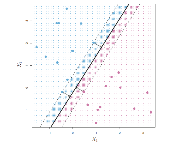
In the figure above, There are two classes of observations, shown in blue and in purple.

The maximal margin hyperplane is shown as a solid straight line.
The margin is the distance from the solid line to either of the dashed lines.
The two blue points and the purple point that lie on the dashed lines are the support vectors
The purple and blue grid indicates the decision rule made by a classiﬁer based on this separating hyperplane.

Problem: Equation (4.2) is a straight hyperplane. Sometimes, it may not separate the datapoints in a clean way.

An example is shown in the following figure. In this case, we cannot exactly separate the two classes.

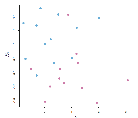
However, as we will see in the next section, we can extend the concept of a separating hyperplane in order to develop a hyperplane that almost separates the classes, using a so-called soft margin. The generalization of the maximal margin classiﬁer to the non-separable case is known as the support vector classiﬁer.

Support Vector Classifier

Support Vector Machine

set.seed(1)
x <- matrix(rnorm(20*2), ncol=2)
y <- c(rep(-1,10), rep(1,10))
x[y==1,] <- x[y==1,] + 1
plot(x, col=(3-y))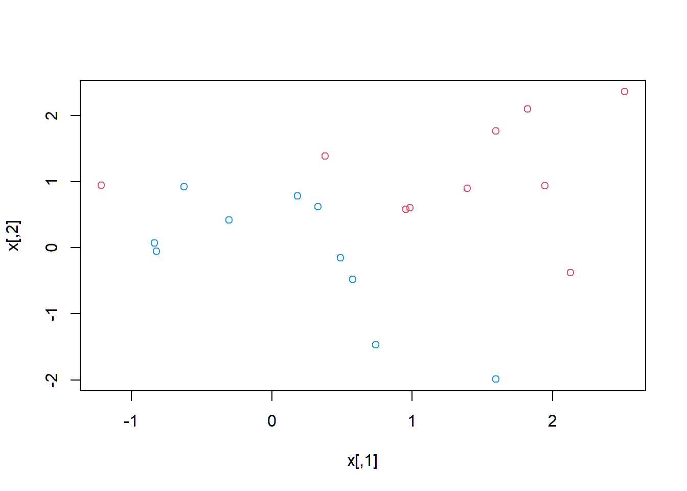

dat <- data.frame(x=x, y=as.factor(y))
library(e1071)

## Warning: package 'e1071' was built under R version 4.4.2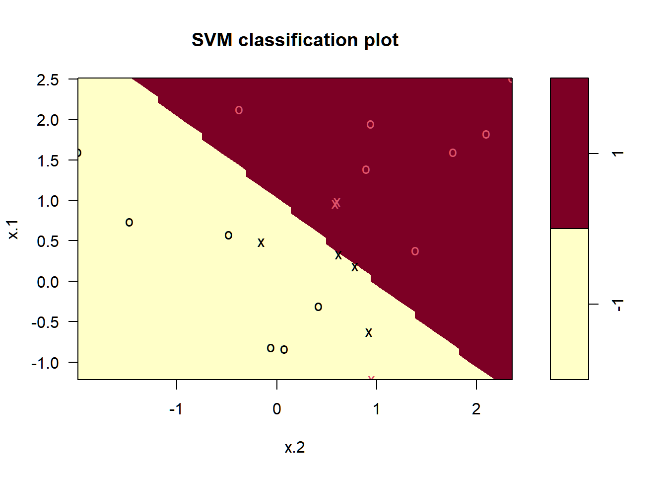

svmfit <- svm(y~., data=dat, kernel="linear", cost=10, scale=FALSE)

plot(svmfit, dat)

The decision boundary between the two classes is linear (because we used the argument kernel="linear").

We can obtain some basic information about the support vector classiﬁer ﬁt using the summary() command:

summary(svmfit)

## 
## Call:
## svm(formula = y ~ ., data = dat, kernel = "linear", cost = 10, scale = FALSE)
## 
## 
## Parameters:
##    SVM-Type:  C-classification 
##  SVM-Kernel:  linear 
##        cost:  10 
## 
## Number of Support Vectors:  7
## 
##  ( 4 3 )
## 
## 
## Number of Classes:  2 
## 
## Levels: 
##  -1 1

This tells us, for instance, that a linear kernel was used with cost=10, and that there were seven support vectors, four in one class and three in the other.

4.1.3 Generalized Additive Models

Definition 4.5 Generalized additive models (GAMs) provide a general framework for extending a standard linear model by allowing non-linear functions of each of the variables, while maintaining additivity.

The following is an extension of multiple linear regression model, which now allows non-linear relationships between each feature ( $X$ ) and the response ( $Y$ )

$y_i = \beta_0 + \sum_{j=1}^pf_j(x_{ij}) + \varepsilon_i$

GAMs for Regression Problems

GAMs for Classification Problems

4.1.4 Tree-based methods

In this section, we describe tree-based methods for regression and classiﬁcation. These involve stratifying or segmenting the predictor space into a number of simple regions.

STAT 142: Introduction to Computational Statistics