2.4 Querying databases in SQL

So far, we have dealt with small data sets that easily fit into your computer’s memory. But what about data sets that are too large for your computer to handle as a whole?

Most data used in class examples are stored in simple flat files (commonly saved in .csv or .xlsx format). Hence, data are organized and stored in a simple file system:

transaction_id	customer_id	date	product_name	quantity	price	amount
001
002
…

Commonly, academic researchers gain data through observational sampling or experiments, and statistical/government agencies still collect data mostly through off-line means (e.g., survey, reports, or census).

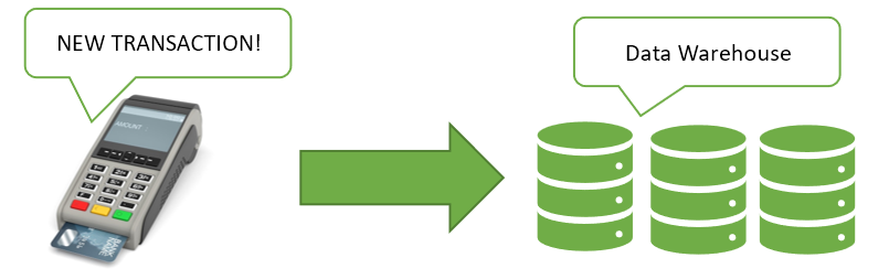
On the other hand, industry and services often get their data on-line from business processes, i.e., from logistical, production, and administrative transactions. For example, sales data may be collected and updated directly from point-of-sales (POS) devices, then stored into some “database” or “datawarehouse”.

Definition 2.5 A database is an organized collection of structured information, or data, typically stored electronically in a computer system.

A database is usually controlled by a database management system (DBMS). Together, the data and the DBMS, along with the applications that are associated with them, are referred to as a database system, often shortened to just database.

When doing analysis from a database, you may only want to extract a part of it, because your computer may not be able to handle if you extract the whole database.

Definition 2.6 Structured Query Language (SQL) is a domain-specific and the standard language used to manage data, especially in a relational database management system.

SQL is used to interact (or “talk”) with relational databases such as SQLite, MySQL, PostgreSQL, Oracle, and Sysbase. This is optimized for certain data arrangements.

When working with large datasets, integrating SQL with R provides an efficient workflow for data manipulation, extraction, and analysis.

2.4.1 Connecting to a Database

There are several ways of running SQL in R. All methods require to connect to a database management system (e.g., MySQL).

However, we do not have access to existing databases. Hence, we shall set-up a simple database in our local machines. That way, we can practice SQL in RStudio without connecting to a formal database.

To set-up an sqlite database in memory, you need to install the RSQLite package.

library(DBI)
library(RSQLite)

To set-up a connection to a database, you need the dbConnect() function from DBI package. In this case, we use dbConnect() to set-up a database in memory.

• First, download the database bank.sqlite to your working directory.

• Now, we connect to SQLite database, which is in our local device.

  bank <- dbConnect(RSQLite::SQLite(), "bank.sqlite")

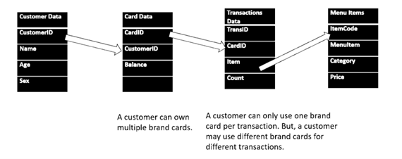
• This database contains 4 tables:

  dbListTables(bank)

  ## [1] "cards"        "customers"    "menu"         "transactions"

  • customers: customer information

  • cards: a list of card ids, customer id of the owner, and remaining balance in the card. A customer may own multiple brand cards.

  • transactions: a list of the items bought in a certain transaction (order). There’s a unique id for each transaction. Take note, transactions require a brand card (which is a reloadable debit card). There may be multiple rows for a single transaction here.

  • menu: a list of item codes, corresponding item names, general category, and price

  

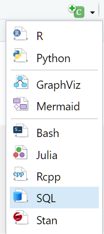
In R Markdown, you may insert an SQL code chunk.

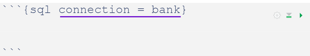
In every SQL code chunk, the connection must be specified. Set connection = bank for our examples.

Now, let’s try extracting all columns from the customer table from this database.

SELECT * FROM customers

ABCDEFGHIJ0123456789

CustomerId <int>	surname <chr>	middle <chr>	given <chr>	sex <fct>	age <int>	bday <chr>	est_income <dbl>
15565701	Ferri	J	Susan	Female	39	1978-06-07	63000
15565706	Akobundu	I	David	Male	35	1982-06-14	56000
15565714	Cattaneo	S	Joseph	Male	47	1970-06-05	73000
15565779	Kent	N	Betty	Female	30	1987-05-18	165000
15565796	Docherty	O	Donald	Male	48	1969-05-27	27000
15565806	Toosey	S	Donald	Male	38	1979-06-26	35000
15565878	Bates	G	Michael	Male	NA	NA	167000
15565879	Riley	P	Lisa	Female	28	1989-06-17	36000
15565891	Dipietro	H	Edward	Male	39	1978-05-27	39000
15565996	Arnold	G	John	Male	44	1973-06-09	117000

Next

123456

...

969

Previous

1-10 of 9,685 rows

Cleaning up

To end a connection from a database, use the R function dbDisconnect() from the DBI package.

dbDisconnect(bank)

In large companies, many users may access a database stored in a cloud server at a single time. It is important that you disconnect from the database especially if the database has connection limits and to avoid possible data corruption.

2.4.2 Simple SQL Queries

There are a large number of SQL major commands, one of which is an SQL query.

A query is a question or inquiry about a set of data. For example, “Tell me how many books there are on computer programming” or “How many Rolling Stones albums were produced before 1980?”.

Generally, it has the following form:

SELECT columns or computations
    FROM table
    WHERE condition
    GROUP BY columns
    HAVING condition
    ORDER BY column [ASC | DESC]
    LIMIT offset,count;

Some notes:

• The SELECT statement should have at least the SELECT clause and FROM clause. All other clauses are optional.

• The order of the clauses within the SELECT query does matter. Do not switch the order of SELECT, FROM, WHERE, GROUP BY, and ORDER BY clauses.

• The language is not case-sensitive, but let us use upper case for keywords.

In the following examples, make sure that you are still connected to the sqlite database, and you write your codes on SQL code chunks.

bank <- dbConnect(RSQLite::SQLite(), "bank.sqlite")

SELECT and FROM

For many of the modern uses of databases, all you’ll need to do with the database is to select some subset of the variables and/or observations from a table, and let some other program manipulate them.

In SQL the, SELECT statement is the workhorse for these operations.

FROM is used to specify the table to query.

SELECT * FROM customers

ABCDEFGHIJ0123456789

CustomerId <int>	surname <chr>	middle <chr>	given <chr>	sex <fct>	age <int>	bday <chr>	est_income <dbl>
15565701	Ferri	J	Susan	Female	39	1978-06-07	63000
15565706	Akobundu	I	David	Male	35	1982-06-14	56000
15565714	Cattaneo	S	Joseph	Male	47	1970-06-05	73000
15565779	Kent	N	Betty	Female	30	1987-05-18	165000
15565796	Docherty	O	Donald	Male	48	1969-05-27	27000
15565806	Toosey	S	Donald	Male	38	1979-06-26	35000
15565878	Bates	G	Michael	Male	NA	NA	167000
15565879	Riley	P	Lisa	Female	28	1989-06-17	36000
15565891	Dipietro	H	Edward	Male	39	1978-05-27	39000
15565996	Arnold	G	John	Male	44	1973-06-09	117000

Next

123456

...

969

Previous

1-10 of 9,685 rows

The asterisk * after SELECT means that you are extracting all columns.

You can also select specific columns only, each separated by comma ,.

SELECT TransID, item
    FROM transactions

ABCDEFGHIJ0123456789

TransId <chr>	item <chr>
10000115634602	BC
10000115634602	FT
10000215634602	Cap
10000215634602	MS
10000315634602	Cap
10000315634602	FT
10000415634602	Cap
10000515634602	GTF
10000515634602	CCF
10000515634602	DDS

Next

123456

...

1000

Previous

1-10 of 10,000 rows

WHERE

Conditional statements can be added via WHERE to filter possible output.

Show all female customers

SELECT * 
    FROM customers
    WHERE Sex = "Female"

ABCDEFGHIJ0123456789

CustomerId <int>	surname <chr>	middle <chr>	given <chr>	sex <fct>	age <int>	bday <chr>	est_income <dbl>
15565701	Ferri	J	Susan	Female	39	1978-06-07	63000
15565779	Kent	N	Betty	Female	30	1987-05-18	165000
15565879	Riley	P	Lisa	Female	28	1989-06-17	36000
15566091	Thomsen	M	Sharon	Female	32	1985-05-09	52000
15566139	Ts'ui	C	Sharon	Female	37	1980-06-02	34000
15566156	Franklin	S	Margaret	Female	44	1973-06-16	119000
15566211	Hsu	K	Patricia	Female	41	1976-05-30	5000
15566251	Ferrari	R	Sharon	Female	37	1980-06-18	64000
15566295	Sanders	B	Jennifer	Female	33	1984-05-08	105000
15566312	Jolly	G	Sharon	Female	42	1975-06-08	152000

Next

123456

...

440

Previous

1-10 of 4,398 rows

Both AND and OR are valid, along with parentheses to affect order of operations.

Extract female aged 50 above, together with all male customers

SELECT * 
    FROM customers
    WHERE (sex = 'Female' AND age >= 50) 
        OR sex = 'Male'

ABCDEFGHIJ0123456789

CustomerId <int>	surname <chr>	middle <chr>	given <chr>	sex <fct>	age <int>	bday <chr>	est_income <dbl>
15565706	Akobundu	I	David	Male	35	1982-06-14	56000
15565714	Cattaneo	S	Joseph	Male	47	1970-06-05	73000
15565796	Docherty	O	Donald	Male	48	1969-05-27	27000
15565806	Toosey	S	Donald	Male	38	1979-06-26	35000
15565878	Bates	G	Michael	Male	NA	NA	167000
15565891	Dipietro	H	Edward	Male	39	1978-05-27	39000
15565996	Arnold	G	John	Male	44	1973-06-09	117000
15566030	Tu	H	Charles	Male	41	1976-05-27	59000
15566111	Estes	T	Richard	Male	39	1978-05-12	56000
15566253	Manning	K	Robert	Male	44	1973-05-14	129000

Next

123456

...

579

Previous

1-10 of 5,784 rows

ORDER BY

To order variables, use the syntax:

ORDER BY var1 {ASC/DESC}, var2 {ASC/DESC}

where the choice of ASC for ascending or DESC for descending is made per variable.

Sort items in menu from most expensive to least expensive

SELECT * FROM menu
    ORDER BY Price DESC

ABCDEFGHIJ0123456789

ItemCode <chr>	MenuItem <chr>	Category <chr>	Price <dbl>
CarM	Caramel Macchiato	Hot Drink	170
ICA	Iced Cafe Americano	Cold Drink	170
DDS	Double Decker Sandwich (Tuna or Chicken)	Bread or Sandwich	170
GTF	Green Tea Frappe	Cold Drink	160
CCF	Chocolate Chip Frappe	Cold Drink	160
Cap	Cappuccino	Hot Drink	150
DMF	Dark Mocha Frappe	Cold Drink	150
ICarM	Iced Caramel Macchiato	Cold Drink	140
CA	Cafe Americano	Hot Drink	130
SHC	Signature Hot Chocolate	Hot Drink	130

Next

123

Previous

1-10 of 21 rows

LIMIT

To control the number of results returned, use LIMIT #.

Show top 10 richest customers”

SELECT * FROM customers
    ORDER BY est_income DESC
    LIMIT 10

ABCDEFGHIJ0123456789

CustomerId <int>	surname <chr>	middle <chr>	given <chr>	sex <fct>	age <int>	bday <chr>	est_income <dbl>
15569274	Pisano	F	Joseph	Male	49	1968-05-28	180000
15616454	Davidson	Q	Donna	Female	34	1983-05-28	180000
15641582	Chibugo	G	Paul	Male	43	1974-06-10	180000
15657957	Hughes	B	Barbara	Female	26	1991-06-06	180000
15670172	Padovesi	B	Patricia	Female	30	1987-06-17	180000
15713621	Mollison	Q	Paul	Male	41	1976-06-15	180000
15741719	DeRose	H	Nancy	Female	40	1977-05-23	180000
15773487	Conway	P	Margaret	Female	31	1986-06-10	180000
15796413	Green	T	Brian	Male	46	1971-06-12	180000
15651983	Fang	N	Helen	Female	56	1961-05-25	179000

1-10 of 10 rows

Aggregate Functions

An aggregate function is a function that performs a calculation on a set of values, and returns a single value.

The most commonly used SQL aggregate functions are:

• MIN() - returns the smallest value within the selected column

• MAX() - returns the largest value within the selected column

• COUNT() - returns the number of rows in a set

• SUM() - returns the total sum of a numerical column

• AVG() - returns the average value of a numerical column

Aggregate functions ignore null values (except for COUNT()).

SELECT COUNT() returns the number of observations.

SELECT COUNT() AS n_transactions 
    FROM transactions

ABCDEFGHIJ0123456789

n_transactions <int>
310970

1 row

Show number of customers that has age

SELECT COUNT() AS n_users, COUNT(age)
    FROM customers

ABCDEFGHIJ0123456789

n_users <int>	COUNT(age) <int>
9685	9637

1 row

Aggregate functions are often used with the GROUP BY clause of the SELECT statement. The GROUP BY clause splits the result-set into groups of values and the aggregate function can be used to return a single value for each group.

Show average income per sex

SELECT sex, AVG(est_income) AS Avg_Income
    FROM customers
    GROUP BY sex

ABCDEFGHIJ0123456789

sex <fct>	Avg_Income <dbl>
Female	77857.31
Male	77236.72

2 rows

The HAVING clause filters a table after aggregation.

Show total count of transaction per items, but only those having total sales greater than 20k.

SELECT item, SUM(count) AS total_sales
    FROM transactions
    GROUP BY item
    HAVING total_sales > 20000

ABCDEFGHIJ0123456789

item <chr>	total_sales <int>
CA	21188
ICarM	21682
MC	21522

3 rows

---

This is only the tip of the SQL iceberg. There are far more advanced commands available, such as the following:

• INSERT: Add new records
• UPDATE: Modify existing data
• DELETE: Remove records
• JOIN: Combine tables

If the database is large enough that you cannot store the entire dataset on your computer, you may need to learn more commands.

2.4.3 Query from Multiple Tables

Recall that the tables in the bank database are connected by some “key variables”.

The transactions table has TransId, CardId, item, and count, but the name of the items cannot be found in this table.

The following is an example query from 2 tables.

SELECT transactions.TransID, transactions.item, menu.MenuItem
    FROM transactions LEFT JOIN menu 
            ON transactions.item = menu.ItemCode

Table 2.1: Displaying records 1 - 10

TransId	item	MenuItem
10000115634602	BC	Brewed Coffee
10000115634602	FT	French Toast
10000215634602	Cap	Cappuccino
10000215634602	MS	Muffin Sandwich (Bacon and Cheese)
10000315634602	Cap	Cappuccino
10000315634602	FT	French Toast
10000415634602	Cap	Cappuccino
10000515634602	GTF	Green Tea Frappe
10000515634602	CCF	Chocolate Chip Frappe
10000515634602	DDS	Double Decker Sandwich (Tuna or Chicken)

We use tableName.columnName to get a column from a specific table.

The LEFT JOIN keyword returns all records from the left table (table1), and the matching records from the right table (table2). The result is 0 records from the right side, if there is no match.

SELECT column_name(s)
    FROM table1
        LEFT JOIN table2
            ON table1.column_name = table2.column_name;

Now, what if we want to find the total number of items sold per item?

Menu items can be found on the menu table, but the number of items sold per transaction can be found on the transactions table.

SELECT  menu.MenuItem, 
        SUM(transactions.count) AS total_sold
    FROM transactions LEFT JOIN menu 
        ON transactions.item = menu.ItemCode
    GROUP BY transactions.item

Table 2.2: Displaying records 1 - 10

MenuItem	total_sold
Banana Bread	8275
Brewed Coffee	18880
Blueberry Cheesecake	14941
Banoffee Pie	16166
Cafe Americano	21188
Chocolate Chip Frappe	13251
Classic Sandwich (Tuna or Chicken)	14693
Cappuccino	14628
Caramel Macchiato	12208
Double Decker Sandwich (Tuna or Chicken)	13501

There are other types of JOIN clauses:

• JOIN: Returns records that have matching values in both tables. Also called an inner join.

• LEFT JOIN: Returns all records from the left table, and the matched records from the right table. This is also recommended if there is many-to-one correspondence between the left and right tables.

• RIGHT JOIN: Returns all records from the right table, and the matched records from the left table. This is also recommended if there is one-to-many correspondence between the left and right tables.

• FULL JOIN: Returns all records when there is a match in either left or right table.

2.4.4 Converting SQL Query to Dataframe

After an SQL Query, they are still not directly useful if we want to perform modelling in R.

The dbGetQuery converts an SQL statement into a dataframe.

customers <- dbGetQuery(conn = bank,
                        "SELECT * 
                        FROM customers")

The return value is a dataframe, where you can now perform any R procedures.

Additional task: convert all tables in bank to dataframes.

Practice Exercises

1. Easy

   Show a table containing number of items per transaction ID.

2. Average

   Recall that a customer may own multiple cards. Show a table with name of all card holders, and another column for the total balance of each customer for all their owned cards. Limit to top 5 customers only.

3. Hard

   What food is commonly paired with “Capuccino”? Show top 3 food items with respective number of transactions.

---

References

• Errickson, J. (n.d.). SQL in R. https://dept.stat.lsa.umich.edu/~jerrick/courses/stat701/notes/sql.html

• W3Schools.com. (n.d.). https://www.w3schools.com/sql/