2.1 Measuring Program Performance
Learning Objective: Apply profiling and timing tools to optimize R code
Before optimizing your code, you need to identify what’s slowing it down. This can be tricky, even for experienced programmers.
Rather than relying on intuition, you should profile your code: measure the run-time of each line of code using realistic inputs.
After identifying bottlenecks, experiment with alternatives to find faster equivalent code. Before exploring optimization techniques, learn microbenchmarking to measure performance differences accurately.
Make sure that the following packages are installed on your devices:
We’ll use profvis for profiling, and bench for microbenchmarking.
2.1.1 Profiling
Programs often suffer from inefficiencies like slow execution or high memory usage, which are hard to detect just by inspecting code.
That’s why we need profiling—it helps identify bottlenecks, guiding optimizations for better performance.
Primitive Way of Measuring Program Runtime
Suppose we have the following codes:
We can quickly measure how long the program was executed by your computer by simply using Sys.time() at the start and end of the program.
Run the whole code chunk simultaneously.
t <- Sys.time()
x <- rnorm(10000000)
samp <- sample(x, size = 100000, replace = FALSE)
runtime <- Sys.time() - t
print(runtime)## Time difference of 0.6720269 secsThe program ran for 0.6720269 seconds.
However, the problem here is that we cannot see the bottleneck yet, and the time is highly dependent on the specification of your computer and current consumption of resources. Estimate may be accurate during the runtime, but not precise.
Profiler in R
In most programming languages, the main tool for analyzing code performance is a profiler.
Rprof() from the utils package uses a simple type known as a sampling or statistical profiler, which pauses execution every few milliseconds to capture the call stack—showing the active function and its callers.
For example, consider the function f() below.
f <- function() {
  pause(0.1)
  g()
  h()
}
g <- function() {
  pause(0.1)
  h()
}
h <- function() {
  pause(0.1)
}
Just for the sake of illustration, the functions do not do anything—except take pauses.
If we profiled the execution of f(), stopping the execution of code every 0.1 s, we’d see a profile like this:
# start profiling of function f(). Store details on a file.
Rprof(filename = "Rprof.out",
      interval = 0.1)
f()
Rprof(NULL) # end profiling
writeLines(readLines("Rprof.out"))
sample.interval=100000
"pause" "f"
"pause" "g" "f"
"pause" "h" "g" "f"
"pause" "h" "f" Each line represents one “tick” of the profiler (0.1 s in this case), and function calls are recorded from right to left: the first line shows f() calling pause(). It shows that the code spends 0.1 s running f(), then 0.2 s running g(), then 0.1 s running h().
With this way of profiling using Rprof(), results may be unclear. We cannot see right away how long a function or command executed. It is better if we visualize it.
Visualizing Profiles
The default profiling resolution is quite small, so if your function takes even a few seconds it will generate hundreds of samples.
That quickly grows beyond our ability to look at directly, so instead of using utils::Rprof() we’ll use the profvis package to visualize aggregates.
profvis is a tool for helping you to understand how R spends its time. It provides a interactive graphical interface for visualizing data from Rprof(), R’s built-in tool for collecting profiling data.
There are two ways to use profvis:
from the Profile menu in RStudio; and
with
profvis::profvis().
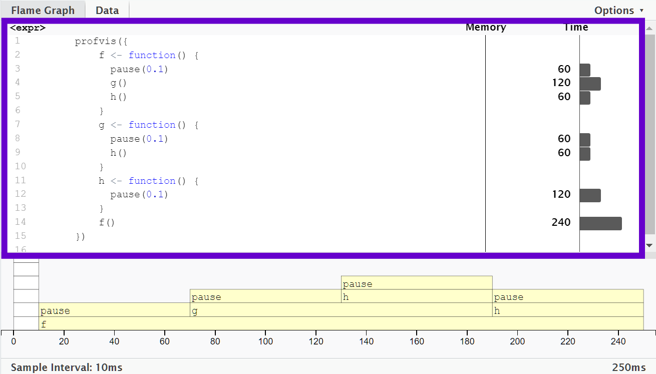
After profiling is complete, profvis will open an interactive HTML document that allows you to explore the results.
The top pane shows the source code, overlaid with bar graphs for memory and execution time for each line of code.
This display gives you a good overall feel for the bottlenecks but doesn’t always help you precisely identify the cause.
Here, for example, you can see that calling
h()takes 60 ms.
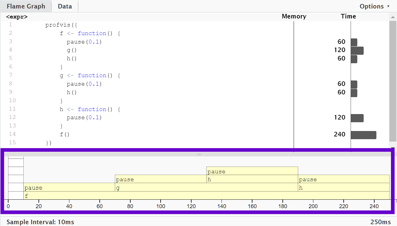
The bottom pane displays a flame graph showing the full call stack.
This allows you to see the full sequence of calls leading to each function, allowing you to see that
h()is called from two different places.In this display you can mouse over individual calls to get more information, and see the corresponding line of source code.
In this example,
f()runs for 240 ms. When it was called,g()was executed afterpause(0.1).g()runs at an average of 120 ms.
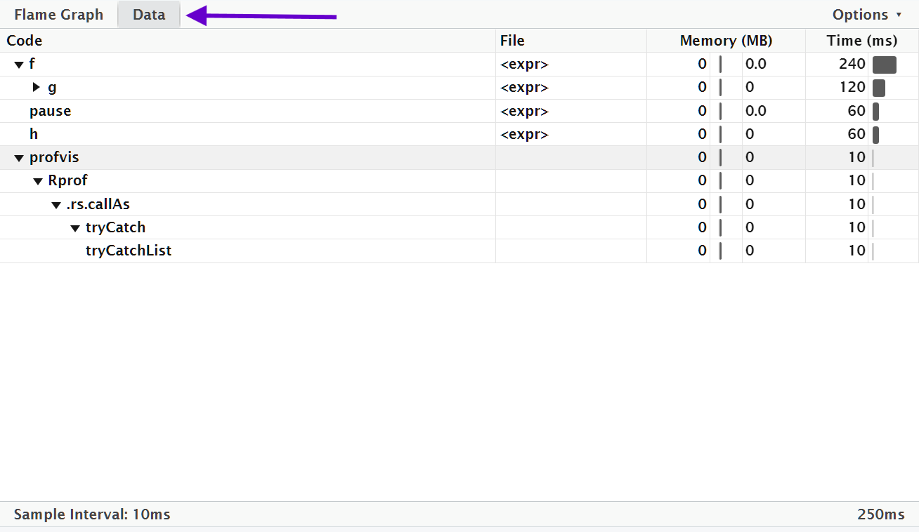
Alternatively, you can use the data tab.
It lets you interactively dive into the tree of performance data.
This is basically the same display as the flame graph (rotated 90 degrees), but it’s more useful when you have very large or deeply nested call stacks because you can choose to interactively zoom into only selected components.
Memory Profiling and Garbage Collection
In programs, we don’t only profile the time execution, but also the memory they occupy.
If an object has no names pointing to it, it gets automatically deleted by the garbage collector (which deletes unused objects in R).
Definition 2.1 In programming, garbage collection (GC) is collecting or gaining memory back which has been allocated to objects but which is not currently in use in any part of our program.
Garbage collection can help in managing memory, but will still take time to process.
In the flame graph, there is a special entry that doesn’t correspond to any of your code: <GC>, which indicates that the garbage collector is running.
If <GC> is taking a lot of time, it’s usually an indication that you’re creating many short-lived objects. For example, take this small snippet of code:
If we profile it, you’ll see that it spent some time in garbage collection.
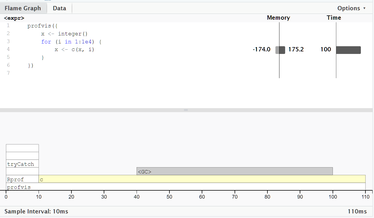
When you see the garbage collector taking up a lot of time in your own code, you can often figure out the source of the problem by looking at the memory column: you’ll see a line where large amounts of memory are being allocated (the bar on the right) and freed (the bar on the left).
Here, the problem arises because of copy-on-modify:
each iteration of the loop creates another copy of
x.the old version of
xwill be unreachable, and gets garbage collected.
GC is not triggered at every iteration, but it happens periodically when R determines that memory needs to be freed.
Specifically:
As
xgrows, more memory is allocated dynamically.The old copies of
xbecome unreachable.When memory pressure builds up, R’s garbage collector runs to reclaim space.
2.1.2 Microbenchmarking
Definition 2.2 A microbenchmark is a measurement of the performance of a very small piece of code, something that might take milliseconds (ms), microseconds (µs), or nanoseconds (ns) to run.
Microbenchmarks are useful for comparing small snippets of code for specific tasks.
A great tool for microbenchmarking in R is the bench package. The bench package uses a high precision timer, making it possible to compare operations that only take a tiny amount of time.
library(bench)For example, the following code compares the speed of two approaches to computing a square root.
expression <bnch_xpr> | min <bench_tm> | median <bench_tm> | itr/sec <dbl> | mem_alloc <bnch_byt> | gc/sec <dbl> |
|---|---|---|---|---|---|
| <bnch_xpr> | 600ns | 700ns | 1059187.4 | 848B | 0 |
| <bnch_xpr> | 3.9µs | 15.1µs | 84273.9 | 848B | 0 |
Note: This result may vary in different devices, which is why we will be using a cloud-based version of R in your exercises.
By default, bench::mark() runs each expression at least once (min_iterations = 1), and at most enough times to take 0.5 s (min_time = 0.5).
expression <bnch_xpr> | min <bench_tm> | median <bench_tm> | itr/sec <dbl> | mem_alloc <bnch_byt> | gc/sec <dbl> |
|---|---|---|---|---|---|
| <bnch_xpr> | 600ns | 700ns | 1135344.41 | 848B | 0 |
| <bnch_xpr> | 3.9µs | 16.3µs | 68648.74 | 848B | 0 |
Interpreting results
bench::mark() returns the results as a tibble, with one row for each input expression, and the following columns:
min,median, anditr/secsummarize the time taken by the expression.Focus on the minimum (the best possible running time) and the median (the typical time).
In this example, you can see that using the special purpose
sqrt()function is faster than the general exponentiation operator.You can visualize the distribution of the individual timings with
plot(). Make sure to install and load the following packages:ggplot2,ggbeeswarm,tidyr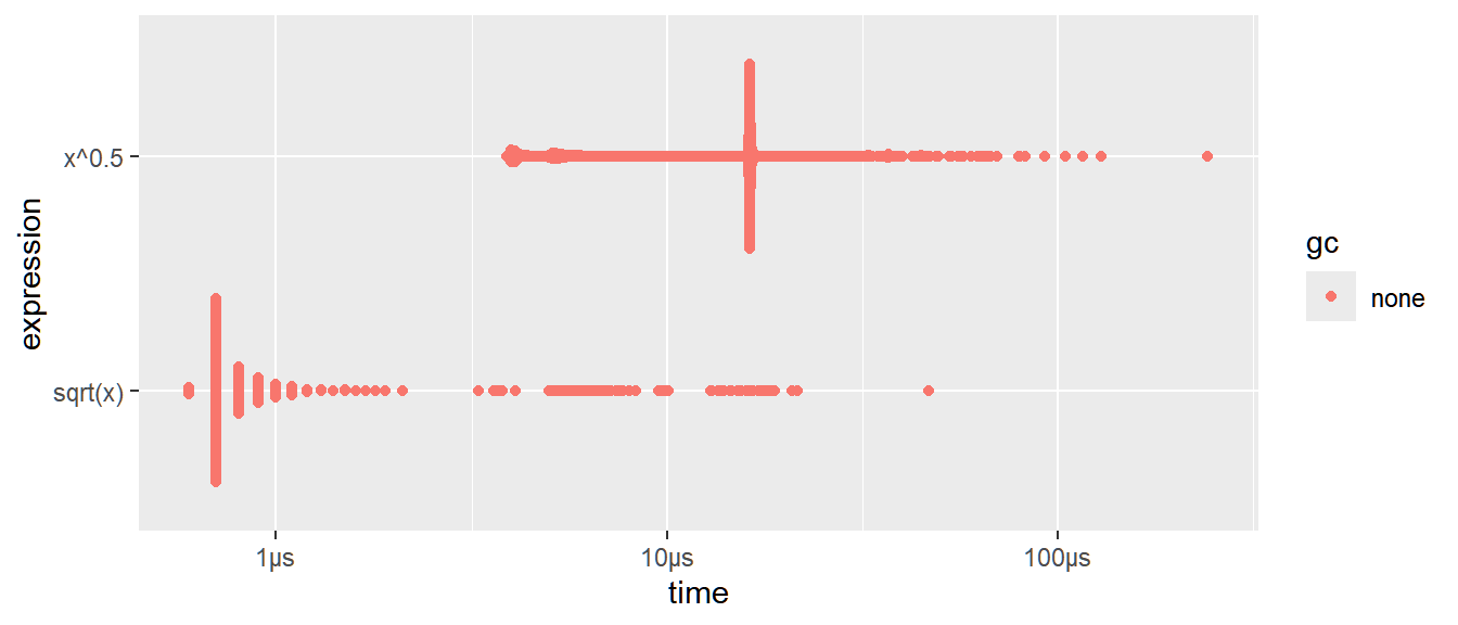
The distribution tends to be heavily right-skewed, which is why you should avoid comparing means. You’ll also often see multimodality because your computer is running something else in the background.
mem_alloctells you the amount of memory allocated by the first run, andn_gc()tells you the total number of garbage collections over all runs. These are useful for assessing the memory usage of the expression.n_itrandtotal_timetells you how many times the expression was evaluated and how long that took in total.n_itrwill always be greater than themin_iterationparameter, andtotal_time will always be greater than themin_time` parameter.
result,memory,time, andgcare list-columns that store the raw underlying data.
Comparing functions with different results
bench::mark function checks that each run returns the same value, which is typically what you want to microbenchmark. On the other hand, if you want to compare the speed of expressions that may return different values each run, set check = FALSE.
# Define two different functions
r_sum <- function(n) {
  sum(1:n)
}
r_product <- function(n) {
  prod(1:n)  # Product of 'n' numbers
}
Note that the results of these two functions are not the same.
## [1] 5050## [1] 9.332622e+157Let’s try microbenchmarking the two functions without checking results by setting check = FALSE.
expression <bnch_xpr> | min <dbl> | median <dbl> | itr/sec <dbl> | mem_alloc <bnch_byt> | gc/sec <dbl> |
|---|---|---|---|---|---|
| <bnch_xpr> | 0.9 | 1.10 | 733982.663 | 8.5625KB | 0 |
| <bnch_xpr> | 853.7 | 862.95 | 1079.287 | 8.015625KB | 0 |
Exercises
Create two functions for obtaining the nth Fibonacci number:
fib_loopthat uses aforloop, andfib_recusing recursion.- Benchmark the two functions for inputs x <- 1:100. Which is faster?
Consider the two search algorithms
linear_searchand `binary_search’.linear_search <- function(arr, target) { for (i in seq_along(arr)) { if (arr[i] == target) { return(i) } } return(-1) }binary_search <- function(arr, target) { left <- 1 right <- length(arr) while (left <= right) { mid <- floor((left + right) / 2) if (arr[mid] == target) { return(mid) } else if (arr[mid] < target) { left <- mid + 1 } else { right <- mid - 1 } } return(-1) }Benchmark the performance of the two functions when finding the string “find_me” in the following vectors:
If the input size is 15, which is faster?
If the input size is 100, which is faster?
If the item to find is found early in the array, which is faster?
If the item to find is found late in the array, which is faster?