Chapter 5 Cross-Validation

In creating statistical models, it is important to evaluate the performance of your model when deployed on new data.

Definition 5.1 Cross-validation is a statistical technique used to assess the performance and generalizability of a predictive model. It involves partitioning the dataset into multiple subsets, training the model on some of these subsets, and validating it on the remaining ones.

The goal is to evaluate how well the model will perform on unseen data and to reduce the risk of overfitting.

---

In this section, we will discuss some cross-validation methods to assess how good the model is in predicting a set of new observations.

There will be three cross-validation methods that will be discussed here:

• Validation Set Approach
• Leave-One-Out Cross-Validation (LOOCV)
• K-Fold Cross-Validation

All of these approaches involve calculating some evaluation metrics or cross-validation estimate. For an overview, here are some of them:

Regression

Let $y_i$ be the actual observed value and let $\hat{y}_i$ be the predicted value computed using $\hat{f}(\text{x}_i)$. The following are possible evaluation metrics in regression. Lower values are better.

• $MSE = \frac{1}{n}\sum_{i=1}^n(y_i-\hat{y}_i)^2$
• $RMSE= \sqrt{\frac{1}{n}\sum_{i=1}^n(y_i-\hat{y}_i)^2}$
• $MAE=\frac{1}{n}\sum_{i=1}^n|y_i-\hat{y}_i|$
• $BIAS=\frac{1}{n}\sum_{i=1}^n(y_i-\hat{y}_i)$

Classification

Suppose we are classifying $y$ into two values (positive or negative). After modelling and predicting the classification of $y$, we have the following confusion matrix.

	Predicted Positive	Predicted Negative
Actual Positive	$TP$	$FN$
Actual Negative	$FP$	$TN$

The following are some evaluation metrics for a binary classification problem. Higher values are better.

• Accuracy: $\frac{TP+TN}{TP + TN+FP+FN}$

• Precision (Positive Predictive Value): $\frac{TP}{TP+FP}$

• Recall (Sensitivity or True Positive Rate): $\frac{TP}{TP + FN}$

• Specificity (True Negative Rate): $\frac{TN}{TN+FP}$

• F1 Score: $2\cdot\frac{Precision\cdot Recall}{Precision + Recall}$

The choice of an evaluation metric will be based on the context of your data. All of these have functions in the Metrics package.

library(Metrics)

In this Chapter, we will focus on cross-validation of models that predict numeric variables, specifically with applications on multiple linear regression only.

---

Validation Set Approach

The train-and-test-set validation, or simply validation set approach, is a a very simple strategy for cross-validation.

The idea is to randomly split the set of observations into two parts, a training set and a test set (also called validation set, or hold-out set).

The model is fit on the training set, and the fitted model is used to predict the responses for the observations in the test set.

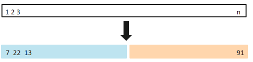
It is common to split the dataframe to 70-30: 70% of the dataset will be used for training the model, and the rest will be used for testing the model.

The resulting test set error rate is typically assessed using MSE or RMSE for quantitative response variables.

set.seed(1)
library(carData)
Anscombe

ABCDEFGHIJ0123456789

	education <int>	income <int>	young <dbl>	urban <int>
ME	189	2824	350.7	508
NH	169	3259	345.9	564
VT	230	3072	348.5	322
MA	168	3835	335.3	846
RI	180	3549	327.1	871
CT	193	4256	341.0	774
NY	261	4151	326.2	856
NJ	214	3954	333.5	889
PA	201	3419	326.2	715
OH	172	3509	354.5	753

Next

123456

Previous

1-10 of 51 rows

validation <- function(formula, data, size = 0.7, criterion){
    
    train_indices <- sample(1:nrow(data), 
                            size = 0.7 * nrow(data))
    
    train_data <- data[train_indices, ]
    test_data  <- data[-train_indices, ]
    
    # Fit model on training data
    lm_fit <- lm(formula, data = train_data)

    # Predict on test data 
    pred <- predict(lm_fit, newdata = test_data)
    
    # Extract the vector of observed y from test data
    obs  <- test_data[[all.vars(formula)[1]]]
    
    # compute and return evaluation metric
    eval <- criterion(obs, pred)
    return(eval)
}

validation(income ~ urban, Anscombe, size = 0.7, Metrics::rmse)

validation(income ~ urban + education, Anscombe, size = 0.7, Metrics::rmse)

validation(income ~ urban + education + young, Anscombe, size = 0.7, Metrics::rmse)

## [1] 552.6391
## [1] 368.039
## [1] 280.6608

---

Leave-One-Out Cross Validation

Leave-one-out cross-validation (LOOCV) is closely related to the validation set approach, but it attempts to address that method’s drawbacks.

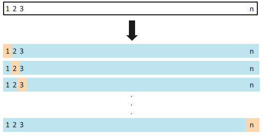
Like the validation set approach, LOOCV involves splitting the set of observations into two parts. However, instead of creating two subsets of comparable size, a single observation $(x_1, y_1)$ is used for the validation set, and the remaining observations ${(x_2, y_2), . . . , (x_n, y_n)}$ make up the training set.

The processes is repeated for all observation to obtain $n$ evaluation metrics, and their average will be obtained for an overall evaluation metric.

Most functions in R already show statistics from LOOCV approach (such as the PRESS), but we will demonstrate the LOOCV approach manually here.

loocv <- function(formula, data, criterion){
    n <- nrow(data)
    eval <- numeric(n)
    for(i in 1:n){
        train_i <- data[-i,]
        test_i  <- data[i,]
        mod_i   <- lm(formula,train_i)
        pred_i  <- predict(mod_i, test_i)
        
        y <- all.vars(formula)[1]
        eval[i] <- criterion(test_i[[y]], pred_i)
    }
    return(mean(eval))
}

loocv(income ~ urban, Anscombe, Metrics::rmse)
loocv(income ~ urban + education, Anscombe, Metrics::rmse)

## [1] 324.9626
## [1] 232.3712

---

k-Fold Cross-validation

An alternative to LOOCV is k-fold CV.

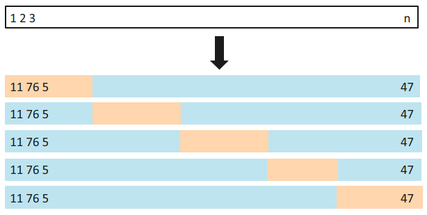
This approach involves randomly dividing the set of observations into $k$ groups, or folds, of approximately equal size.

The first fold is treated as a validation set, and the method is fit on the remaining $k − 1$ folds. This process results in $k$ estimates of the evaluation metric. The k-fold cross validation estimate is computed as the average of the $k$ metrics.

LOOCV is a special case of k-Fold CV, where $k=n$.

kfold <- function(formula, data, k = 10, criterion){
    n <- nrow(data)
    # Assigning folds
    folds <- sample(rep(1:k, length.out = n))
    
    # Loop
    eval <- numeric(k)
    for (i in 1:k){
        #splitting the dataset
        train <- data[folds!=i,]
        test  <- data[folds==i,]
        
        # modelling
        mod     <- lm(formula, data = train)
        pred    <- predict(mod, test)
        y <- all.vars(formula)[1]
        eval[i] <- criterion(test[[y]], pred)
    }
   
    return(mean(eval))
}

kfold(income ~ urban, data = Anscombe, k = 10,      Metrics::rmse)

kfold(income ~ urban + young,data = Anscombe, k = 10, Metrics::rmse)

## [1] 389.2178
## [1] 432.4814

Example/Exercise: Model performance through the years

In this exercise, we explore if a model created in 1952 is still useful for prediction as years go by using some exploratory data analysis. Install and load the package gapminder for this exercise.

1. Create a new function lm_validate that inputs the following:

   • formula: the formula to be used

   • train: training set to be used

   • test: test set to be used

   • criterion: the evaluation metric function to be used

   This should perform the Validation Set Approach for linear regression, but you will have more control which data will be used for training and testing.

2. Load the dataset gapminder included in the package gapminder.

   library(gapminder)
   gapminder

   ABCDEFGHIJ0123456789

   country <fct>	continent <fct>	year <int>	lifeExp <dbl>	pop <int>	gdpPercap <dbl>
   Afghanistan	Asia	1952	28.80100	8425333	779.4453
   Afghanistan	Asia	1957	30.33200	9240934	820.8530
   Afghanistan	Asia	1962	31.99700	10267083	853.1007
   Afghanistan	Asia	1967	34.02000	11537966	836.1971
   Afghanistan	Asia	1972	36.08800	13079460	739.9811
   Afghanistan	Asia	1977	38.43800	14880372	786.1134
   Afghanistan	Asia	1982	39.85400	12881816	978.0114
   Afghanistan	Asia	1987	40.82200	13867957	852.3959
   Afghanistan	Asia	1992	41.67400	16317921	649.3414
   Afghanistan	Asia	1997	41.76300	22227415	635.3414

   Next

   123456

   ...

   171

   Previous

   1-10 of 1,704 rows

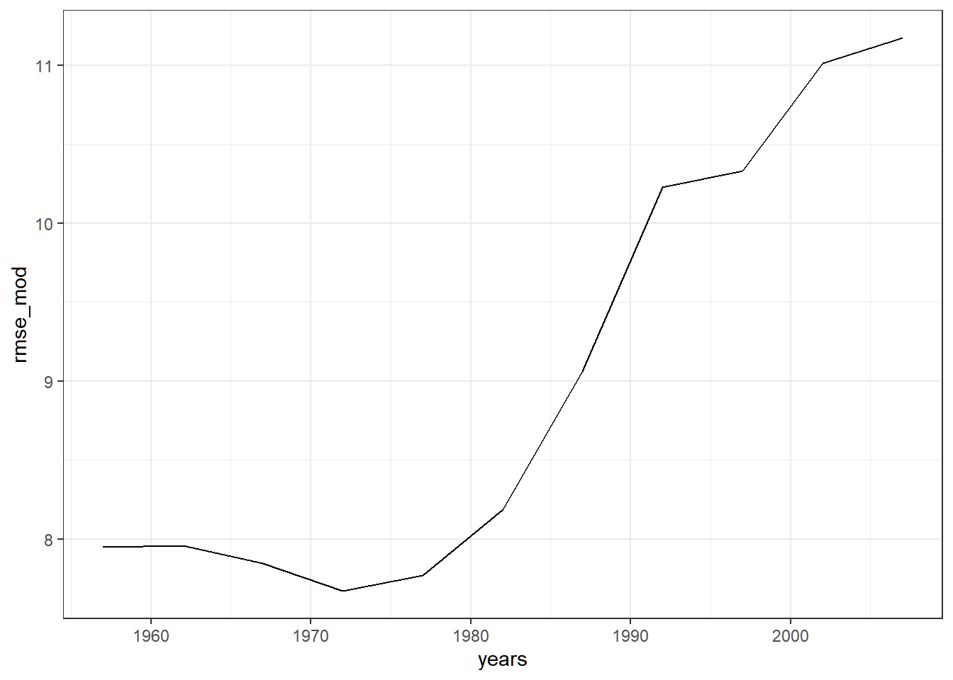
3. Filter the dataset to show only values in 1952. Fit a linear regression model that predicts lifeExp using log(gdpPercap) and pop.

4. Using the model in (3) and the function in (1), predict the lifeExp of each country per year, and show how the RMSE changes through the years. It should look something like this:

   

---

References

Much of the content of this chapter is derived from An Introduction to Statistical Learning with Applications in R (James, Witten, Hastie, & Tibshirani, 2013)

For further reading, you may explore the the cv package by John Fox and Georges Monette:

• Introduction to cv package. https://cran.r-project.org/web/packages/cv/vignettes/cv.html

• Cross-validating Model Selection. https://cran.r-project.org/web/packages/cv/vignettes/cv-selection.html