3.4 Bootstrapping and Resampling Methods

Resampling methods play a crucial role in modern statistics, allowing us to estimate properties of a population by repeatedly sampling from observed data.

One of the most powerful resampling techniques is the bootstrap, introduced by Efron (1979). The bootstrap is an example of Monte Carlo approach that provides a framework for statistical inference without relying on strong parametric assumptions.

This chapter explores bootstrap methods, their theoretical foundations, and their applications in R.

Motivation for resampling

Traditional statistical inference relies on theoretical sampling distribution of a statistic or a point estimator, which may not always be applicable, especially when:

• the underlying distribution is unknown or difficult to estimate.

• the sample size is small, making asymptotic results unreliable.

• non-standard parameters (e.g., medians, percentiles) are of interest.

Resampling methods, such as the bootstrap, allow us to approximate the sampling distribution of a statistic using computational techniques rather than relying on mathematical derivations.

Bootstrapping: The General Idea

Definition 3.14 Bootstrapping, first introduced by Efron (1982), is a computationally intensive method that resamples the data to make inferences using estimates obtained about parameters that describe the target population (Mooney & Duval, 1993).

There are three forms of bootstrapping which differ primarily in how the probability distribution is estimated.

• Nonparametric (resampling)

• Parametric (simulation)

• Semiparametric (adding noise, or still model based)

Most people who have heard of bootstrapping have only heard of the so-called nonparametric or resampling bootstrap.

We use semiparametric or parametric bootstrapping when we know more information about the data or statistic of interest.

In the succeeding sections, both nonparametric and parametric bootstrapping will be discussed.

---

3.4.1 Parametric bootstrapping

Parametric bootstrapping assumes that the data comes from a known distribution with some parameters.

For example:

• Poisson or Negative Binomial for counts

• Exponential or Gamma for waiting time

• Normal for other continuous data

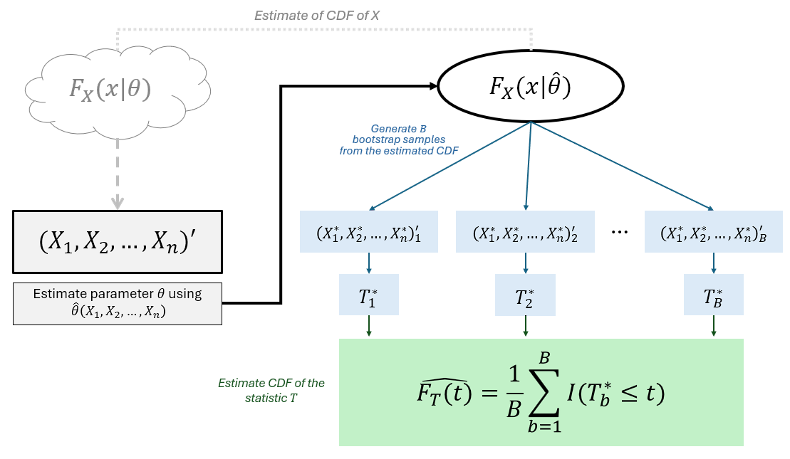
The general steps for parametric bootstrapping is as follows:

1. Let $(X_1,X_2,..., X_n)'$ be a random sample from a known parametric distribution $F(x|\theta)$, where $\theta$ is a parameter.

2. Suppose $\hat{\theta}$ is a point estimator of the parameter $\theta$. Estimate the parameter $\theta$ using the random sample $(X_1,X_2,..., X_n)'$.

3. Using the estimated $\hat{\theta}$, generate a random sample $(X_1^*, X_2^*,...,X_n^*)$ from the distribution $F(x|\hat{\theta})$.

4. Calculate the statistic of interest $T^*$ using the the new sample data $(X_1^*, X_2^*,...,X_n^*)$.

5. Perform 3 and 4 $B$ times to obtain $B$ bootstrap values $T*$.

6. The bootstrap estimate of the sampling distribution of $T^*$ is

   $$F_{\hat{\theta}}(t)=\frac{1}{B}\sum_{b=1}^B I(T^*\leq t)$$

   The bootstrap estimate of the standard error of the statistic $T^*$ is as follows:

   $$\widehat{se}_{boot}(T^*) = \sqrt{ \frac{1}{B-1}\sum_{b=1}^B\left(T^*_b-\overline{T^*}\right)^2}$$

   where $\overline{T^*}=\frac{1}{B}\sum_{b=1}^BT^*_b$ is the the sample mean of the statistic $T^*$ after $B$ bootstrap resamples.

---

Bootstrap Mean from Normal

Assume that we have a sample data $X_1,X_2, ..., X_n$ drawn from a normal distribution $N(\mu, \sigma^2)$.

Suppose we are interested in understanding the sampling distribution of the sample mean $\bar{X}$.

The following dataset sampled from a Normally distributed population:

x <- c(6.5, 3.3, 5.4, 3.2, 3.8, 2.5, 3.2, 5.5, 8.1, 6.3)

Estimate the mean and standard deviation from the sample

mu_hat    <- mean(x)
sigma_hat <- sd(x)

Generate many bootstrap samples from $N(\hat{\mu},\hat{\sigma}^2)$, and compute the sample mean for each.

B <- 1000
bootstrap_means <- numeric(B)
for(b in 1:B){
    x.star <- rnorm(10, mu_hat, sigma_hat)
    bootstrap_means[b] <- mean(x.star)
}

We can now visualize the bootstrap distribution of the sample mean.

ggplot(data.frame(bootstrap_means), aes(bootstrap_means))+
    geom_histogram(aes(y = ..density..), bins = 20) +
    theme_bw()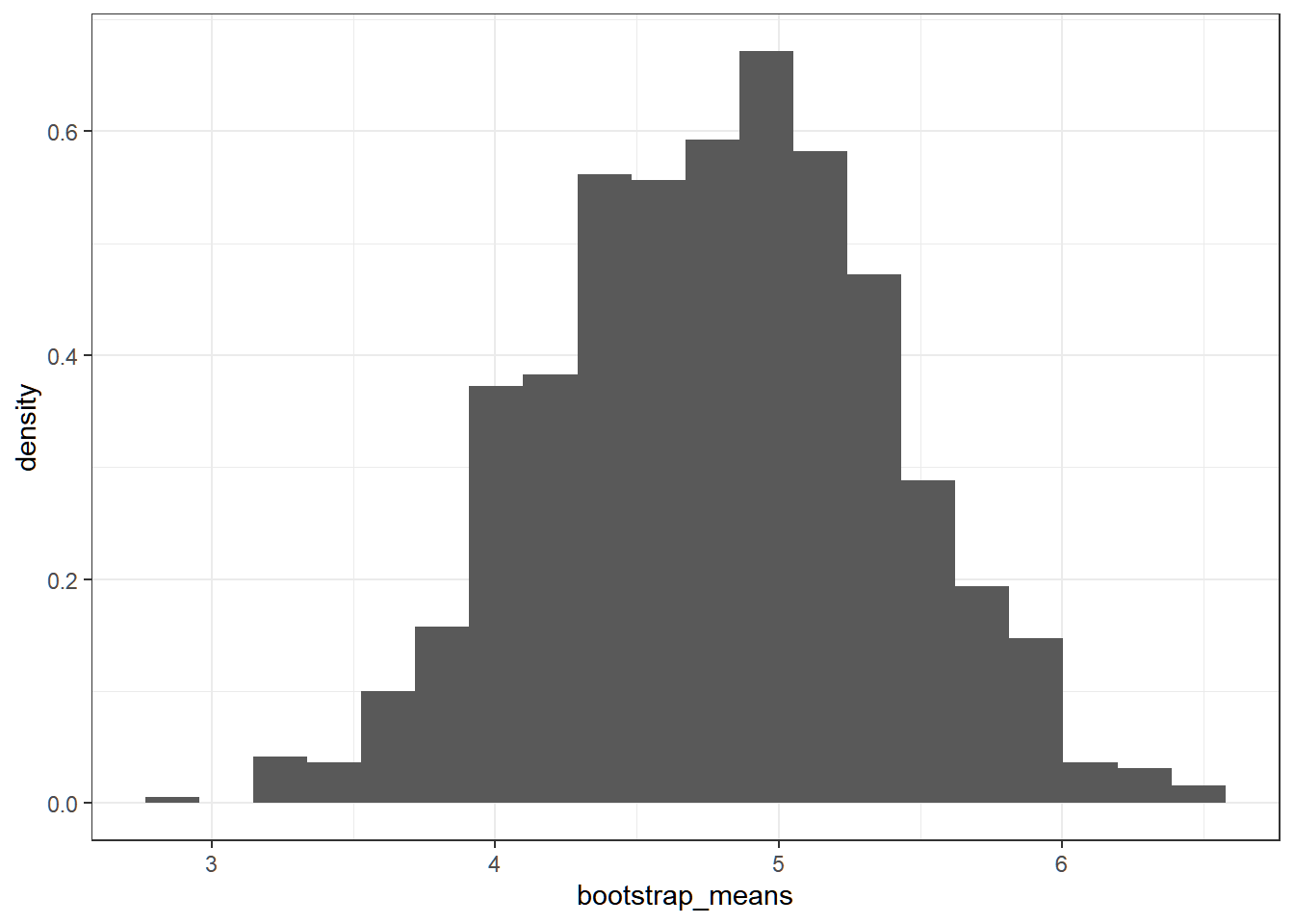

The histogram of bootstrap sample means approximates the sampling distribution of the sample mean.

As a comparison, we know that $\bar{X}\sim N(\mu,\sigma^2/n)$ assuming $\mu$ and $\sigma^2$ are known. Now, plotting the empirical CDF of $\bar{X}$ from the generated bootstrap samples and the CDF of $\bar{X} \sim N(\hat{\mu},\widehat{\sigma^2}/n)$:

ggplot(data.frame(xbar = bootstrap_means),
       aes(x = xbar))+
    geom_function(fun = pnorm, args = list(mean = mu_hat, sd = sigma_hat/sqrt(10)), aes(color = "cdf"))+
    stat_ecdf(aes(color = "ecdf")) +
    ggtitle("CDF of Xbar of a sample from Normal") +
    scale_color_manual( values = c("cdf" = "blue", "ecdf" = "red")) +
    theme_bw()+
    theme(legend.title = element_blank()) +
    ylab(TeX("$P(X\\leq x)$"))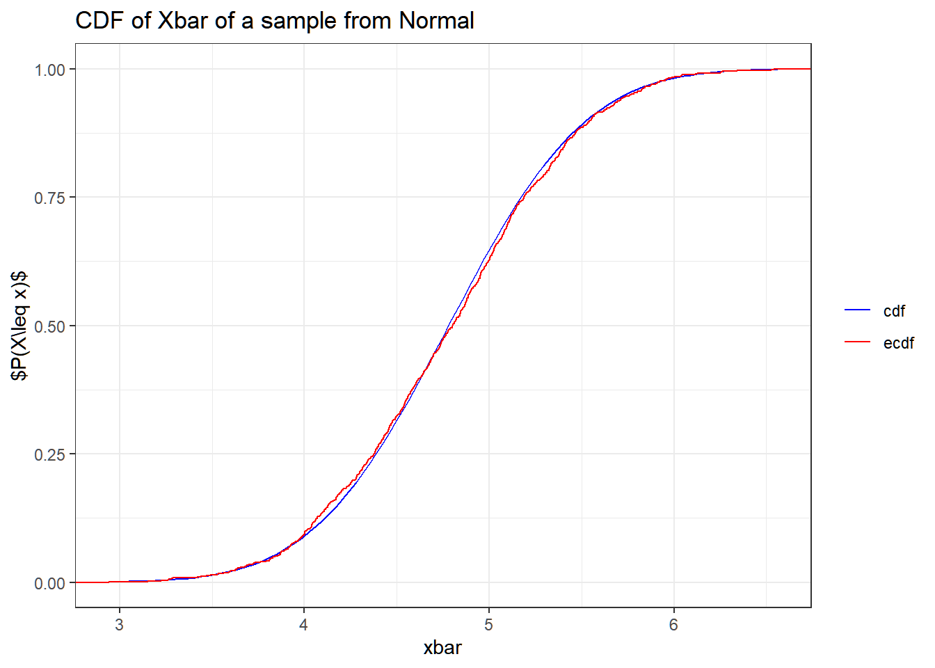

Even if the theoretical distribution is known, the bootstrap provides an empirical check and is especially valuable if the sample size is small or if the sampling distribution is unknown.

Inference

1. Using the bootstrap means, we can estimate the standard error of the sample mean.

   sd(bootstrap_means)

   ## [1] 0.5955176

2. Using the bootstrap distribution, we can compute confidence intervals for the mean $\mu$.

   quantile(bootstrap_means, probs = c(0.025, 0.975))

   ##     2.5%    97.5% 
   ## 3.633327 5.922261

   The 95% confidence interval obtained from the quantiles of the bootstrap distribution provides an intuitive measure of uncertainty around the sample mean. The method above is called the Percentile Bootstrap, which has the following formula:

   $$(\hat{\theta}^*_{(\alpha/2)},\hat{\theta}^*_{(1-\alpha/2)},)$$

   Alternatively, one can also youse Reverse Percentile Interval (or basic bootstrap) to obtain a confidence interval

   $$(2\hat{\theta}-\hat{\theta}^*_{(1-\alpha/2)}, 2\hat{\theta}-\hat{\theta}^*_{(\alpha/2)})$, where $\hat{\theta}^*_(q)$ is the $q^{th}$ percentile of the bootstrapped statistic $\hat{\theta}$$

Bootstrap Means of Count Data

The cd4 dataset from the boot package contains the following variables:

• baseline : The CD4 counts (in 100’s) on admission to the trial.

• oneyear The CD4 counts (in 100’s) after one year of treatment with the new drug.

More details about the dataset:

CD4 cells are carried in the blood as part of the human immune system. One of the effects of the HIV virus is that these cells die. The count of CD4 cells is used in determining the onset of full-blown AIDS in a patient.

In this study of the effectiveness of a new anti-viral drug on HIV, 20 HIV-positive patients had their CD4 counts recorded and then were put on a course of treatment with this drug. After using the drug for one year, their CD4 counts were again recorded.

library(boot)
cd4*100

ABCDEFGHIJ0123456789

	baseline <dbl>	oneyear <dbl>
1	212	247
2	435	461
3	339	526
4	251	302
5	404	636
6	510	593
7	377	393
8	335	409
9	410	488
10	335	381

Next

12

Previous

1-10 of 20 rows

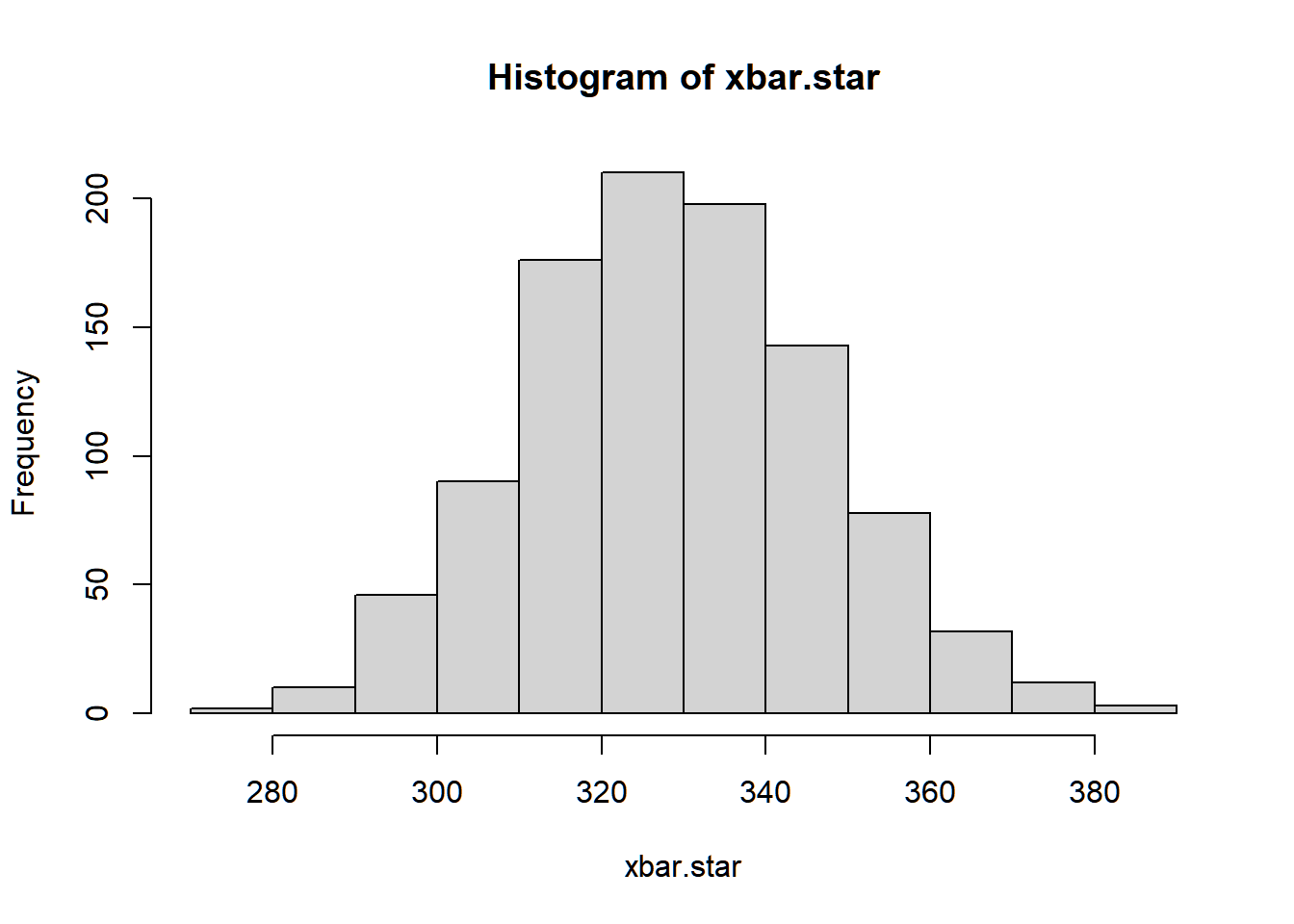
Count data is often modelled with either Poisson or Negative Binomial distribution.

For this example, the observed variance of baseline CD4 counts (6570.59) is much greater than the observed mean (328.80)

var(cd4$baseline*100)
mean(cd4$baseline*100)

## [1] 6570.589
## [1] 328.8

It is more logical to use Negative Binomial when variance is inflated, since Poisson has the same mean and variance $\lambda$.

Recall that Negative Binomial models the number of failures before $r$ number of successes, given probability of success $p$.

A reparameterized version of this uses mean $\mu$ and overdispersion $r$ (sometimes $\theta$ specially if non-integer) as parameters.

Note the following relations:

$$\mu = \frac{r(1-p)}{p}\\ \sigma^2 = \frac{r(1-p)}{p^2}\\ \theta = \frac{\mu^2}{\sigma^2-\mu}$$

If $\mu$ and $\sigma^2$ are estimated using $\bar{X}$ and $s^2$, then

$$\hat{\theta} = \frac{\bar{X}^2}{s^2-\bar{X}}$$

x_bar <- mean(cd4$baseline*100)
s_sq  <- var(cd4$baseline*100)
theta_hat <- x_bar^2/(s_sq-x_bar)

Now that we have the estimated parameters of the negative binomial distribution, we can now have bootstrap estimate of the sampling distribution of the sample mean $\bar{X}$.

The rnbinom generates a negative binomial random numbers, with arguments

• mu = $\mu$ (the mean)
• size = $\theta$ (if as dispersion parameter) or $r$ (if as target number of successes)

B <- 1000
xbar.star <- numeric(B)
n.star <- length(cd4$baseline*100)
for(b in 1:B){
    set.seed(b)
    x.star <- rnbinom(n = n.star, size = theta_hat, mu = x_bar)
    xbar.star[b] <- mean(x.star)
}

hist(xbar.star)

---

Exercise 3.7 (Resampling from Normal Distribution) Suppose we have the following dataset sampled from Normal distribution:

y <- c(8.2, 4.9, 10.8, 6.7, 6.4, 10.0, 8.1, 8.3, 12.5, 10.6)

Obtain a bootstrap estimate of the standard error of the sample variance using this dataset.

Use $B = 1000$, and set seed 1 to 1000 for each bootstrap sample.

You may use var for the computation of sample variance.

---

3.4.2 Nonparametric bootstrapping

Suppose we want to obtain an inference about a parameter $\theta$, which can be estimated using the statistic $\hat{\theta}=T(X_1,X_2,...X_n)'$.

The problem is that our inference can be limited if we do not know the the parent population of $X_1,X_2,...X_n$, hence, the sampling distribution of $\hat{\theta}$ cannot be derived.

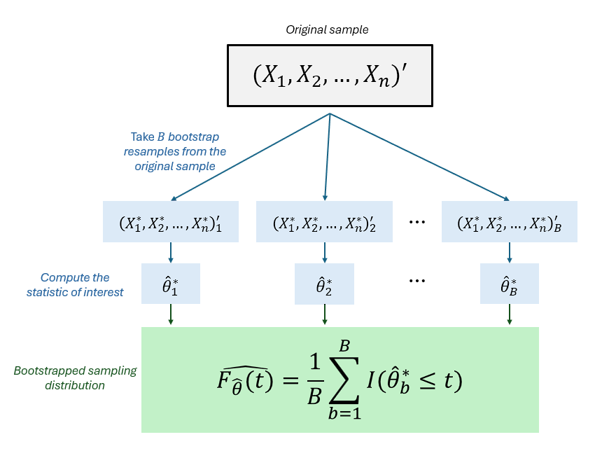
A general outline of the estimation procedure for any population parameter $\theta$ using the nonparametric bootstrap is summarized below:

1. Let $(X_1,X_2,...,X_n)′$ be a sample obtained from the target population using respondent-driven sampling.

2. A bootstrap sample $(X^*_1,X^*_2,...,X^*_n)'$ is obtained by drawing a random sample of size $n$ with replacement from the original sample

3. Compute bootstrap statistic $\hat{\theta}^∗$ using the bootstrap sample as $\hat{\theta}^∗=T(X^*_1,X^*_2,...,X^*_n)'$

4. Repeat 2 and 3 $B$ times to obtain $B$ bootstrap statistics. We denote the bootstrap statistic at the $b^{th}$ iteration as $\hat{\theta}^*_b$

5. The nonparametric bootstrap estimate of the CDF of $\hat{\theta}$ (or the sampling distribution of $\hat{\theta}$) is the empirical distribution function of the bootstrap estimates:

   $$\begin{align} \hat{F}(t)&= \frac{\# \text{ of }\hat{\theta}_bs \leq t}{B}\\ &=\frac{1}{B}\sum_{b=1}^B I(\hat{\theta_b}\leq t) \end{align}$$ Note that the bootstrap estimate of the standard error of $\hat{\theta}$ is the sample standard deviation of the bootstrap estimates $\hat{\theta}^*_1,\hat{\theta}^*_2,...,\hat{\theta}^*_B$

   $$\widehat{se}_{boot}(\hat{\theta}) = \sqrt{\frac{1}{B-1}\sum_{b=1}^B(\hat{\theta}_b^*-\bar{\hat{\theta}^*})^2}$$

   where $\bar{\hat{\theta}^*}=\frac{1}{B}\sum_{b=1}^B\hat{\theta}^*_b$, the average of the bootstrap estimates.

Nonparametric Bootstrap Means

Now, suppose we have the following data, but the distribution of the population is unknown.

samp <- c(12.5, 18.4, 15.1, 4.3, 22.3, 15.2, 6.1, 14.0, 13.8, 9.5, 3.4, 4.2, 2.7, 5.5, 3.5)

For this case, we don’t know the sampling distribution of the sample mean, since the population distribution is unknown, and we cannot use central limit theorem due to low sample size ($n=15$).

This is when nonparametric bootstrap becomes useful. Sampling with replacement from the original dataset creates a “pseudopopulation”.

B <- 1000
xbar.star <- numeric(B)

for (b in 1:B){
    set.seed(b)
    samp.star <- sample(samp, size = 15, replace = T)
    xbar.star[b] <- mean(samp.star)
}

Alternatively, without using a for loop:

xbar.boot <- replicate(B, mean(sample(samp, replace = T)))

ggplot(data = data.frame(xbar.boot), aes(xbar.boot)) + 
  geom_histogram(aes(y=..density..), fill = "#1F78B4") + 
  geom_density(alpha=.5, fill = "#A6CEE3") +
  theme_light()

## `stat_bin()` using `bins =
## 30`. Pick better value with
## `binwidth`.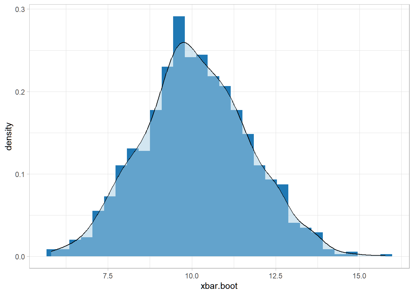

Inference

Suppose we want to test:

$$Ho: \mu=\mu_0 \quad \text{vs} \quad Ha: \mu\neq\mu_0$$

and the estimator for $\mu$ is the sample mean $\bar{X}$.

For our example, let $\mu_0=9$

1. Confidence interval

   One way is to construct a $100(1-\alpha)\%$ confidence interval, and check if $\mu_0$ is in the interval.

   quantile(xbar.star, c(0.025, 0.975))

   ##      2.5%     97.5% 
   ##  7.065833 13.234167

   Since $\mu_0=9$ is in the 95% confidence interval, at $\alpha=0.05$ level of significance, we do not reject $Ho$. There is no sufficient evidence to conclude that $\mu\neq9$

2. Using P-value

   The p-value is defined as the probability of obtaining a test statistic that is more extreme than the one observed, assuming that the null hypothesis is true.

   For our example, the observed statistic is $\bar{X}=10.0333$. From the different values $\bar{X}_b^*$, we want to find the proportion of bootstrap estimates that are more extreme than the observed $\bar{X}$:

   $$p=\frac{\#\left\{|\bar{X}^*_b-9|\geq|\bar{X}-9|\right\}}{B}$$

   Using the bootstrap estimates,

   mean(abs(xbar.star - 9) >= abs(mean(samp)-9))

   ## [1] 0.615

   Comparing with result of t-test:

   t.test(samp, mu = 9)

   ## 
   ##  One Sample t-test
   ## 
   ## data:  samp
   ## t = 0.63706, df = 14, p-value = 0.5344
   ## alternative hypothesis: true mean is not equal to 9
   ## 95 percent confidence interval:
   ##   6.554402 13.512265
   ## sample estimates:
   ## mean of x 
   ##  10.03333

   Again, we cannot use the t-test directly unless normality is assumed.

Bootstrap Estimate of the standard error of Pearson’s r

Bootstrapping is not restricted to univariate case. To add, we can also explore the properties of any statistic, not necessarily for an estimator of a distribution’s parameter.

The following is a data of Efron and Tibshirani:

lsat <- c(576, 635, 558, 578, 666,
          580, 555, 661, 651, 605,
          653, 575, 545, 572, 594)

gpa <- c(3.39, 3.30, 2.81, 3.03, 3.44,
         3.07, 3.00, 3.43, 3.36, 3.13,
         3.12, 2.74, 2.76, 2.88, 2.96)
(lawschool <- data.frame(lsat, gpa))

ABCDEFGHIJ0123456789

lsat <dbl>	gpa <dbl>
576	3.39
635	3.30
558	2.81
578	3.03
666	3.44
580	3.07
555	3.00
661	3.43
651	3.36
605	3.13

Next

12

Previous

1-10 of 15 rows

The lawschool data is a random sample of size $n=15$ from $N=82$ American law schools participating in a large study of admission practices

• lsat the average score of the class on a national law school admision test

• gpa the average undergraduate grade-point average for the class

We want to explore the correlation of GPA and LSAT score using the Pearson’s coefficient of correlation $r$

$$r = \frac{\frac{1}{n-1}\sum(X_i-\bar{X})(Y_i-\bar{Y})}{S_xS_y}$$

where $S_x$ and $S_y$ are the sample standard deviations of the $X$ and $Y$ variables respectively.

The following is the correlation coefficient using the dataset:

corr(lawschool)

## [1] 0.7763745

Again, we are interested in the sampling distribution of $r$ to make an inference about the population correlation $\rho$.

Suppose we cannot assume the joint distribution of $(LSAT,GPA)'$. The following is an algorithm that uses bootstrap to estimate the distribution and standard error of the Pearson Coefficient of Correlation $r$.

r.boot <- function(x, y, B){
    # storing x and y in a single data frame for easy resampling
    data <- data.frame(x, y) 
    
    # length of the data
    n <- nrow(data)         
    
    # vector that stores the bootstrap estimates r
    r.star <- numeric(B)          
    
    for (b in 1:B){
        set.seed(b)
        # resampling procedure
        data.boot <- data[sample(c(1:n),n, replace = T),]  
        # computation of the  correlation
        r.star[b] <- cor(data.boot$x, data.boot$y)         
    }
    return(r.star)
}

set.seed(100)
r.star <- r.boot(lsat,gpa, 2000) 

hist(r.star)

sd(r.star)

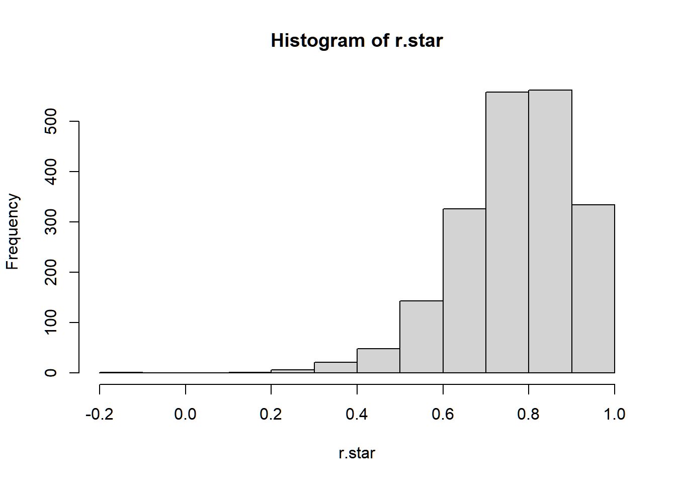
## [1] 0.1336672

Exercise 3.8 Recall the cd4 dataset. The difference of CD4 counts after 1 year is given by:

diff <- (cd4$oneyear - cd4$baseline)*100

Obtain a 95% percentile confidence bootstrap estimate for the mean of the differences based on nonparametric bootstrap procedure with $B = 2000$.

Interpret the results.

3.4.3 Semiparametric Bootstrap

When population distribution is unknown, but some relationship or model can be assumed, then we can perform a semiparametric bootstrap procedure.

For example, in classical simple linear regression: the Gaussian model assumes that the errors are normally distributed. That is:

$$y_i = \beta_0+\beta x_i +\varepsilon_i\\ \varepsilon_i \overset{iid}{\sim} N(0,\sigma^2)$$

This further implies the distribution of the OLS estimator:

$$\hat{\beta} = \frac{\sum(y_i-\bar{y})(x_i-\bar{x})}{\sum(x_i-\bar{x})^2} \sim N\left(\beta,\frac{\sigma^2}{\sum(x_i-\bar{x})^2}\right)$$

And finally,

$$\frac{\hat{\beta}-\beta}{\widehat{se(\hat{\beta})}} \sim t_{\nu = n-2}$$

where $\widehat{se(\hat{\beta})}=\sqrt{MSE/\sum(x_i-\bar{x})^2}$

Inferences about the coefficients $\beta$ that are based on the T-distribution (e.g. confidence intervals and t-test p-values) will be invalid if the error terms are not normally distributed. This is where a semiparametric bootstrap method will be useful.

Residual Bootstrap in Regression

The following is an algorithm that implements residual bootstrapping

1. Fit the model using the original data to obtain:

   • the estimates $\hat{\beta}_0=\bar{y}-\hat{\beta}\bar{x}$ and $\hat{\beta}=\sum_{i=1}^n\frac{(y_i-\bar{y})(x_i-\bar{x})}{\sum_{i=1}^n(x_i-\bar{x})^2}$

   • the fitted values $\hat{y}_i=\hat{\beta}_0 + \hat{\beta}x_i$

   • the residuals $e_i=y_i-\hat{y}_i$

2. From the residuals $(e_1,...,e_n)$, sample with replacement to obtain bootstrap residuals $(e_1^*,e_2^*,...e_n^*)$.

3. Using the resampled residuals, create a synthetic response variable $y_i^*=\hat{y}_i+e_i^*$

4. Using the synthetic response variable $y_i^*$, refit the model to obtain bootstrap estimate of the coefficient $\hat{\beta}_0^*$ and $\hat{\beta}^*$

5. Repeat 2,3,4 $B$ times to obtain $B$ values of $\hat{\beta}_0^*$ and $\hat{\beta}^*$.

Exercise 3.9 Create a function boot_reg that implements residual bootstrap in simple linear regression. It should have the following parameters:

• y - a vector of the dependent variable

• x - a vector of the independent variable

• alpha - the $\alpha$ level of significance

• B - the number of bootstrap replicates

It should have the following as output in a list:

• reg_table: a data frame with the following layout: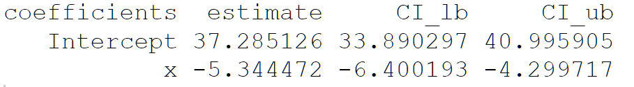

  

• intercept_vec:vector of estimated coefficients $\hat{\beta_0}^*$

• betahat_vec: vector of estimated coefficients $\hat{\beta}^*$

Apply this function on the vectors mtcars$mpg and mtcars$wt as the dependent and independent variables respectively, with $B = 2000$ and $\alpha=0.05$

---

Why does bootstrapping work?

The bootstrap is remarkable because resampling gives us a decent estimate on how the point estimate (or any statistic) might vary.

The bootstrap is roughly based on the law of large numbers:

for large enough data sets, the empirical distribution will be a good approximation of the true distribution

Visually, it says that the histogram of the data should approximate the density of the true distribution.

---

---

Other resampling methods

• Permutation tests, one of the earliest resampling methods (Fisher, 1935), test whether a treatment has zero effect by comparing the observed statistic to those from randomly shuffled data. By breaking any real association through reshuffling, a null distribution is generated. The observed statistic is then evaluated against this distribution. If all permutations are used, it’s an exact test; if many random shuffles are used, it’s a randomization test.

• The jackknife, introduced by Quenouille (1949) and named by Tukey (1958), estimates variance and bias using a leave-one-out approach. For a dataset of $n$ observations, $n$ estimates are computed, each omitting one observation, and then aggregated. This is computationally demanding for large $n$, but it still paved the way for the development of the bootstrap.

• Evaluating a model on the same data used to train it leads to overly optimistic performance estimates. A better approach is to split the data into training and testing sets. Cross-validation improves this by repeatedly splitting the data in different ways, training and testing each time, and averaging the results to get a more reliable performance estimate. More on this in Chapter 5.

---

References

Outline of this chapter is adapted from Stat 142 handouts of Asst. Prof. Xavier Javines Bilon. Other references are the following:

• Efron, B., & Tibshirani, R. (1994). An introduction to the Bootstrap. CRC Press.

• Davison, A. C.; Hinkley, D. V. (1997). Bootstrap methods and their application. Cambridge Series in Statistical and Probabilistic Mathematics. Cambridge University Press.

• James, G., Witten, D., Hastie, T., & Tibshirani, R. (2013a). An Introduction to Statistical Learning. In Springer texts in statistics. https://doi.org/10.1007/978-1-4614-7138-7